
Chapter 7: Vector Spaces and Linear Independence
Chapter Objectives
Upon completing this chapter, you will be able to:
- Understand the formal definition of a vector space and its underlying axioms, recognizing how sets of data like images or text embeddings can form vector spaces.
- Analyze sets of vectors to determine if they are linearly independent or dependent, and articulate the implications for feature selection and redundancy.
- Implement algorithms in Python to compute the span of a set of vectors, find the basis for a vector space, and determine its dimension.
- Design feature transformations by changing basis, and understand how this process is fundamental to dimensionality reduction techniques like Principal Component Analysis (PCA).
- Evaluate the properties of different bases and their impact on the stability and efficiency of machine learning algorithms.
- Apply the concepts of vector spaces and linear independence to solve practical problems in natural language processing (NLP) and computer vision.
Introduction
In the landscape of modern artificial intelligence, data is the new oil, and linear algebra is the refinery. While previous chapters introduced vectors and matrices as tools for storing and manipulating data, this chapter delves into their fundamental structure: the vector space. A vector space is not merely a collection of vectors; it is a universe with its own rules of geometry and interaction. Understanding this universe is paramount for an AI engineer, as it provides the theoretical bedrock for many of the most powerful techniques in machine learning. From the way Google’s search engine understands query semantics to how Netflix recommends your next favorite movie, the principles of vector spaces are at play.
This chapter will guide you through the abstract yet immensely practical concepts of linear combinations, span, linear independence, and basis. These are not just mathematical curiosities; they are the language we use to describe and manipulate high-dimensional feature spaces. We will explore how a set of vectors can span a space, creating a landscape of all possible feature combinations. We will learn to identify linear independence, a crucial property for building efficient and robust models by eliminating redundant information. Most importantly, we will uncover the concept of a basis, which acts as a coordinate system for our data, and see how choosing the right basis can reveal hidden patterns and simplify complex problems—the very essence of dimensionality reduction and feature engineering. By the end of this chapter, you will not only see data as tables of numbers but as points and directions within a structured geometric space, empowering you to build more intuitive, efficient, and powerful AI systems.
Technical Background
The journey from raw data to actionable insight in machine learning is one of transformation. We transform images, text, and sensor readings into numerical representations—vectors—that our algorithms can process. The mathematical environment where these vectors live, interact, and are transformed is a vector space. This section lays the foundational theory of vector spaces, providing the essential language and concepts for understanding the geometry of data.
The Formalism of Vector Spaces
At its core, a vector space is a collection of objects called vectors, which can be added together and multiplied (“scaled”) by numbers, called scalars. For a collection \(V\) to be formally considered a vector space over a field of scalars \(F\) (for our purposes, \(F\) will almost always be the set of real numbers, \(\mathbb{R}\)), it must satisfy a specific set of ten axioms. These rules ensure that the arithmetic operations within the space behave in a consistent and predictable manner, much like the rules of standard arithmetic.
Let \(u\), \(v\), and \(w\) be vectors in \(V\), and let \(c\) and \(d\) be scalars in \(\mathbb{R}\). The axioms are:
- Closure under addition: If \(u\) and \(v\) are in \(V\), then \(u + v\) is also in \(V\). (The space is self-contained for addition.)
- Commutativity of addition: \(u + v = v + u\). (Order doesn’t matter when adding.)
- Associativity of addition: \((u + v) + w = u + (v + w)\). (Grouping doesn’t matter when adding.)
- Existence of a zero vector: There exists a vector \(\mathbf{0}\) in \(V\) such that \(v + \mathbf{0} = v\) for all \(v\) in \(V\).
- Existence of additive inverses: For every \(v\) in \(V\), there is a vector \(-v\) in \(V\) such that \(v + (-v) = \mathbf{0}\).
- Closure under scalar multiplication: If \(c\) is a scalar and \(v\) is in \(V\), then \(cv\) is also in \(V\). (The space is self-contained for scaling.)
- Distributivity of scalar multiplication with respect to vector addition: \(c(u + v) = cu + cv\).
- Distributivity of scalar multiplication with respect to scalar addition: \((c + d)v = cv + dv\).
- Associativity of scalar multiplication: \(c(dv) = (cd)v\).
- Existence of a multiplicative identity: \(1v = v\), where \(1\) is the multiplicative identity scalar.
Axioms of a Vector Space
| Axiom Category | Axiom Name | Mathematical Statement | Intuitive Meaning |
|---|---|---|---|
| Addition | Closure under Addition | If u, v ∈ V, then u + v ∈ V | Adding two vectors in the space results in a vector still within that space. |
| Commutativity | u + v = v + u | The order of vector addition doesn’t matter. | |
| Associativity | (u + v) + w = u + (v + w) | The grouping of vectors in addition doesn’t matter. | |
| Zero Vector | ∃ 0 ∈ V such that v + 0 = v | There’s a neutral element for addition that doesn’t change vectors. | |
| Additive Inverse | ∀ v ∈ V, ∃ –v ∈ V such that v + (-v) = 0 | Every vector has an opposite that cancels it out to the zero vector. | |
| Scalar Multiplication |
Closure under Scalar Multiplication | If c ∈ ℝ, v ∈ V, then cv ∈ V | Scaling a vector keeps it within the same vector space. |
| Distributivity (Vector) | c(u + v) = cu + cv | Scaling a sum of vectors is the same as summing the scaled vectors. | |
| Distributivity (Scalar) | (c + d)v = cv + dv | Scaling by a sum of scalars is the same as summing the scaled vectors. | |
| Associativity | c(dv) = (cd)v | The grouping of scalars in multiplication doesn’t matter. | |
| Identity Element | 1v = v | Scaling a vector by 1 leaves it unchanged. |
While these axioms may seem abstract, they are what give vector spaces their power. They guarantee that the familiar geometric intuitions we have in 2D or 3D space (represented by \(\mathbb{R}^2\) and \(\mathbb{R}^3\)) can be generalized to higher dimensions. For an AI engineer, this is critical. A 1024-pixel grayscale image can be thought of as a single vector in \(\mathbb{R}^{1024}\). A word embedding might be a vector in \(\mathbb{R}^{300}\). The axioms of vector spaces assure us that we can meaningfully operate on these high-dimensional objects—adding them, scaling them, and measuring distances between them—in a mathematically sound way.
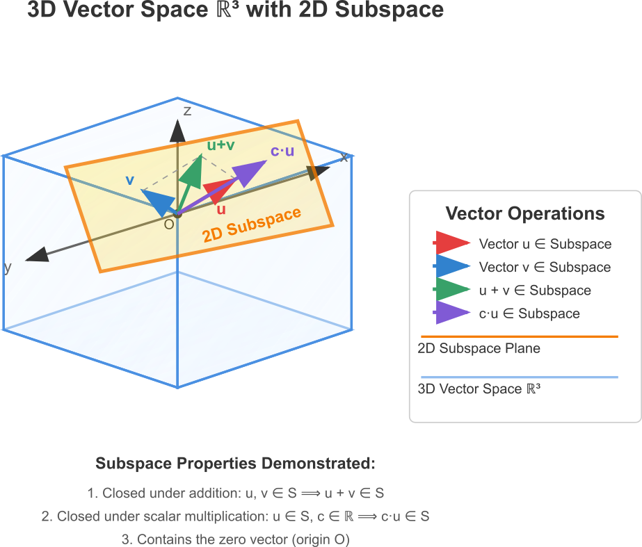
A subspace is a special subset of a vector space that is, itself, a vector space. For a subset \(W\) of a vector space \(V\) to be a subspace, it only needs to satisfy three conditions: it must contain the zero vector, it must be closed under vector addition, and it must be closed under scalar multiplication. For instance, in the 3D space \(\mathbb{R}^3\), a plane passing through the origin is a subspace. It is a 2D vector space existing within a 3D one. In machine learning, the set of all possible solutions to a system of linear equations often forms a subspace, which is a key concept in understanding the behavior of models like linear regression.
Linear Combinations and Span: The Building Blocks of a Space
With the rules of the vector space established, we can begin to construct things within it. The most fundamental operation for building new vectors from existing ones is the linear combination. Given a set of vectors \(\{v_1, v_2, …, v_k\}\) in a vector space \(V\), a linear combination of these vectors is any vector \(v\) of the form:v=c1v1+c2v2+…+ckvk
where \(c_1, c_2, …, c_k\) are scalars. Think of the vectors \(v_i\) as fundamental ingredients and the scalars \(c_i\) as the quantities in a recipe. A linear combination is the result of mixing these ingredients according to the recipe.
This simple idea leads to a powerful concept: the span. The span of a set of vectors \(\{v_1, v_2, …, v_k\}\) is the set of all possible linear combinations of those vectors. It represents every point in the space that can be reached using only those vectors as building blocks.
- If we take a single non-zero vector \(v_1\) in \(\mathbb{R}^3\), its span is a line passing through the origin. We can only move forward and backward along that single direction.
- If we take two vectors \(v_1\) and \(v_2\) that do not point in the same direction, their span is a plane passing through the origin. We can combine them to reach any point on that flat surface.
- If we add a third vector \(v_3\) that does not lie on the plane spanned by \(v_1\) and \(v_2\), their span becomes the entire \(\mathbb{R}^3\) space.
The span of a set of vectors \(S\) is always a subspace of the original vector space \(V\). We say that the set \(S\) spans or generates this subspace. In machine learning, the columns of a feature matrix can be seen as vectors. The span of these column vectors, known as the column space of the matrix, represents the entire range of possible outputs that a linear model can produce. If a target output vector lies outside this column space, it is impossible for the linear model to predict it perfectly; the model can only find the closest possible vector within its span. This is the geometric interpretation of why linear regression finds a “best fit” line or plane.
graph TB
    subgraph Process of Building with Vectors
        direction LR
        0[Vectors ] ---
        A[("Start with a set of<br>vectors {<b>v</b>₁, <b>v</b>₂, ..., <b>v</b>ₖ}")];
        B{{"Choose a set of<br>scalars {c₁, c₂, ..., cₖ}"}};
        C["Perform scalar multiplication:<br>c₁<b>v</b>₁, c₂<b>v</b>₂, ..., cₖ<b>v</b>ₖ"];
        D["Sum the results:<br><b>v</b> = c₁<b>v</b>₁ + c₂<b>v</b>₂ + ... + cₖ<b>v</b>ₖ"];
        E[("<b>v</b> is a <br><b>Linear Combination</b>")];
    end

    subgraph The Resulting Space
        F{"Repeat for <i>all possible</i><br>scalar choices"};
        G[("The set of <b>ALL</b> possible<br>linear combinations")];
        H(("<b>Span</b>({<b>v</b>₁, <b>v</b>₂, ..., <b>v</b>ₖ})<br><i>A Subspace</i>"));
    end

    A --> B;
    B --> C;
    C --> D;
    D --> E;
    E --> F;
    F --> G;
    G --> H;

    classDef start-node fill:#283044,stroke:#283044,stroke-width:2px,color:#ebf5ee;
    classDef process-node fill:#78a1bb,stroke:#78a1bb,stroke-width:1px,color:#283044;
    classDef decision-node fill:#f39c12,stroke:#f39c12,stroke-width:1px,color:#283044;
    classDef data-node fill:#9b59b6,stroke:#9b59b6,stroke-width:1px,color:#ebf5ee;
    classDef end_node fill:#2d7a3d,stroke:#2d7a3d,stroke-width:2px,color:#ebf5ee;

    class A,G start-node;
    class C,D process-node;
    class B,F decision-node;
    class E,H end_node;
Linear Independence: The Essence of Efficiency
The concept of span tells us what we can build, but it doesn’t tell us if our set of building blocks is efficient. This is where linear independence comes in. A set of vectors \(\{v_1, v_2, …, v_k\}\) is said to be linearly independent if the only way to form the zero vector as a linear combination is by using all zero scalars. That is, the equation:c1v1+c2v2+…+ckvk=mathbf0
has only one solution: \(c_1 = c_2 = … = c_k = 0\).
If there is any other solution where at least one scalar is non-zero, the set is said to be linearly dependent.
What does this mean intuitively?
- Linear Independence: Each vector in the set provides unique directional information. No vector can be expressed as a linear combination of the others. The set is non-redundant. Removing any vector from the set will shrink the space it spans.
- Linear Dependence: At least one vector in the set is redundant. It can be constructed from the others. For example, if \(v_3 = 2v_1 – v_2\), then the set \(\{v_1, v_2, v_3\}\) is linearly dependent because we can write \(2v_1 – v_2 – v_3 = \mathbf{0}\), where the scalars \((2, -1, -1)\) are not all zero. The vector \(v_3\) adds no new “direction” or information that wasn’t already contained in the span of \(\{v_1, v_2\}\).
In AI and data science, linear independence is a proxy for informational efficiency. When we perform feature engineering, we aim to create features that are as linearly independent as possible. If two features are highly correlated (nearly linearly dependent), they are providing redundant information. This can make models less stable, harder to interpret, and computationally more expensive to train. Techniques like Principal Component Analysis (PCA) are explicitly designed to find a new set of features (principal components) that are perfectly linearly independent (in fact, orthogonal), ensuring that each new feature captures a unique dimension of variance in the data.
Comparing Span and Linear Independence
| Aspect | Span | Linear Independence |
|---|---|---|
| Core Question | What can we build with a set of vectors? | Is the set of vectors efficient and non-redundant? |
| Focus | The entire subspace (e.g., line, plane, volume) that can be reached. It’s about reachability. | The relationship between the vectors within the set. It’s about redundancy. |
| Definition | The set of all possible linear combinations of the vectors. | A set where the only linear combination resulting in the zero vector is the trivial one (all scalars are zero). |
| Effect of Adding a Dependent Vector |
The span does not change. The new vector was already reachable. | The set immediately becomes linearly dependent. |
| Effect of Adding an Independent Vector |
The span expands into a higher dimension. | The set may remain linearly independent (if the new vector is outside the existing span). |
| AI Implication | Defines the entire range of possible outputs for a linear model (the column space). | Identifies redundant features. An independent set of features is efficient and desirable for model stability. |
Note: A common method to check for linear independence of \(n\) vectors in \(\mathbb{R}^n\) is to form a matrix \(A\) with these vectors as its columns. The vectors are linearly independent if and only if the determinant of \(A\) is non-zero. More generally, for \(k\) vectors in \(\mathbb{R}^n\), they are linearly independent if and only if the rank of the matrix \(A\) is equal to \(k\).
Basis and Dimension: The Coordinate System of Data
We can now combine the concepts of span and linear independence to define the most important concept in this chapter: the basis. A basis for a vector space \(V\) is a set of vectors \(B\) that satisfies two conditions:
- \(B\) is linearly independent.
- \(B\) spans \(V\).
A basis is therefore a maximally efficient set of building blocks for a space. It contains the minimum number of vectors required to build every other vector in the space, and it does so without any redundancy. Think of a basis as the fundamental axes of a coordinate system. In standard 2D space (\(\mathbb{R}^2\)), the most common basis is the set of vectors \(\{\mathbf{i}, \mathbf{j}\}\), where \(\mathbf{i} = [1, 0]\) and \(\mathbf{j} = [0, 1]\). This set is linearly independent (you can’t write \(\mathbf{i}\) as a multiple of \(\mathbf{j}\)) and it spans all of \(\mathbb{R}^2\) (any vector \([x, y]\) can be written as \(x\mathbf{i} + y\mathbf{j}\)).
While a vector space can have infinitely many different bases, a remarkable and crucial theorem states that every basis for a given vector space has the same number of vectors. This unique number is called the dimension of the vector space.
- The dimension of \(\mathbb{R}^2\) is 2.
- The dimension of \(\mathbb{R}^3\) is 3.
- The dimension of \(\mathbb{R}^n\) is \(n\).
- A plane through the origin in \(\mathbb{R}^3\) is a subspace of dimension 2.
- A line through the origin in \(\mathbb{R}^3\) is a subspace of dimension 1.
The dimension is the intrinsic “degrees of freedom” of the space. In machine learning, the number of features in a dataset corresponds to the dimension of the space in which the data points live. A dataset with 100 features corresponds to a collection of points in a 100-dimensional vector space. The goal of dimensionality reduction is to find a lower-dimensional subspace that captures most of the “important” information from the original high-dimensional space. This is achieved by finding a new basis for the data and discarding the basis vectors that correspond to the least important directions of variation. The concepts of basis and dimension provide the formal language to describe and execute this process.

Practical Examples and Implementation
Theoretical understanding is the map, but practical implementation is the journey. In this section, we translate the abstract concepts of vector spaces, independence, and basis into concrete Python code. Using standard scientific computing libraries like NumPy and Matplotlib, we will explore how to test these properties, compute them, and visualize them, connecting the mathematics directly to AI development workflows.
Implementing Vector Space Operations with NumPy
NumPy is the cornerstone of numerical computation in Python. Its core data structure, the ndarray, is a perfect representation of a vector or a matrix. Basic vector space operations are straightforward.
import numpy as np

# Define two vectors in R^3
v1 = np.array([1, 2, 3])
v2 = np.array([4, 5, 6])

# Define two scalars
c1 = 2
c2 = -0.5

# --- Vector Addition (u + v) ---
# This demonstrates closure under addition, as the result is another NumPy array of the same shape.
sum_vector = v1 + v2
print(f"Vector Addition (v1 + v2): {sum_vector}")

# --- Scalar Multiplication (c*v) ---
# This demonstrates closure under scalar multiplication.
scaled_vector = c1 * v1
print(f"Scalar Multiplication (c1 * v1): {scaled_vector}")

# --- Linear Combination (c1*v1 + c2*v2) ---
# The fundamental building block of vector spaces.
linear_combination = c1 * v1 + c2 * v2
print(f"Linear Combination (c1*v1 + c2*v2): {linear_combination}")

# --- Zero Vector ---
# The additive identity in R^3
zero_vector = np.zeros(3)
print(f"Zero Vector + v1: {zero_vector + v1}")

# --- Additive Inverse (-v) ---
inverse_vector = -v1
print(f"v1 + (-v1): {v1 + inverse_vector}")
This code snippet demonstrates that the fundamental axioms of a vector space are naturally handled by NumPy’s element-wise operations, allowing us to work with high-dimensional vectors as easily as with single numbers.
Testing for Linear Independence
Determining whether a set of vectors is linearly independent is a critical task. As discussed, this is equivalent to checking the rank of a matrix whose columns are the vectors in question. The rank of a matrix is the dimension of the vector space spanned by its columns (or rows), which in this context means the number of linearly independent vectors in the set.
Let’s test two sets of vectors in \(\mathbb{R}^3\): one dependent and one independent.
import numpy as np

# --- Case 1: A Linearly Dependent Set ---
# v3 is a linear combination of v1 and v2 (v3 = v1 + v2)
v1_dep = np.array([1, 0, 1])
v2_dep = np.array([-2, 1, 0])
v3_dep = np.array([-1, 1, 1]) # v1_dep + v2_dep

# Create a matrix from these vectors (as columns)
A_dep = np.array([v1_dep, v2_dep, v3_dep]).T
print("Matrix for dependent set (A_dep):\n", A_dep)

# Calculate the rank
rank_dep = np.linalg.matrix_rank(A_dep)
num_vectors_dep = A_dep.shape[1]

print(f"\nNumber of vectors: {num_vectors_dep}")
print(f"Rank of the matrix: {rank_dep}")

if rank_dep < num_vectors_dep:
    print("Conclusion: The set of vectors is Linearly DEPENDENT.")
else:
    print("Conclusion: The set of vectors is Linearly INDEPENDENT.")

print("-" * 40)

# --- Case 2: A Linearly Independent Set ---
# These vectors point in fundamentally different directions (the standard basis)
v1_indep = np.array([1, 0, 0])
v2_indep = np.array([0, 1, 0])
v3_indep = np.array([0, 0, 1])

A_indep = np.array([v1_indep, v2_indep, v3_indep]).T
print("Matrix for independent set (A_indep):\n", A_indep)

rank_indep = np.linalg.matrix_rank(A_indep)
num_vectors_indep = A_indep.shape[1]

print(f"\nNumber of vectors: {num_vectors_indep}")
print(f"Rank of the matrix: {rank_indep}")

if rank_indep < num_vectors_indep:
    print("Conclusion: The set of vectors is Linearly DEPENDENT.")
else:
    print("Conclusion: The set of vectors is Linearly INDEPENDENT.")
In Case 1, the rank (2) is less than the number of vectors (3), correctly identifying the redundancy. In Case 2, the rank (3) equals the number of vectors (3), confirming their independence. This rank test is a computationally robust and general method that works for any number of vectors in any dimensional space.
Visualizing Span and Basis
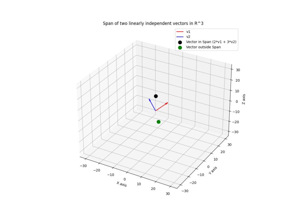
Abstract concepts like span become much clearer with visualization. Let’s visualize the span of two vectors in 3D space using Matplotlib.
import numpy as np
import matplotlib.pyplot as plt
from mpl_toolkits.mplot3d import Axes3D

# Define two linearly independent vectors in R^3
v1 = np.array([1, 2, 1])
v2 = np.array([-2, 1, 2])

# Generate a grid of scalars to create linear combinations
c1_range = np.linspace(-10, 10, 25)
c2_range = np.linspace(-10, 10, 25)
c1_grid, c2_grid = np.meshgrid(c1_range, c2_range)

# Calculate the linear combinations for each point on the grid
# We use np.outer to help construct the plane
span_x = np.outer(v1[0], c1_grid) + np.outer(v2[0], c2_grid)
span_y = np.outer(v1[1], c1_grid) + np.outer(v2[1], c2_grid)
span_z = np.outer(v1[2], c1_grid) + np.outer(v2[2], c2_grid)

# Plotting
fig = plt.figure(figsize=(12, 9))
ax = fig.add_subplot(111, projection='3d')

# Plot the plane (the span of v1 and v2)
ax.plot_surface(span_x, span_y, span_z, alpha=0.5, cmap='viridis', rstride=10, cstride=10)

# Plot the basis vectors
origin = [0, 0, 0]
ax.quiver(*origin, *v1, color='r', length=10, normalize=True, label='v1', arrow_length_ratio=0.2)
ax.quiver(*origin, *v2, color='b', length=10, normalize=True, label='v2', arrow_length_ratio=0.2)

# A vector that lies within the span
v_in_span = 2 * v1 + 3 * v2
ax.scatter(v_in_span[0], v_in_span[1], v_in_span[2], color='k', s=100, label='Vector in Span (2*v1 + 3*v2)')

# A vector that lies outside the span
v_out_span = np.array([5, -5, -5])
ax.scatter(v_out_span[0], v_out_span[1], v_out_span[2], color='g', s=100, label='Vector outside Span')

ax.set_xlabel('X axis')
ax.set_ylabel('Y axis')
ax.set_zlabel('Z axis')
ax.set_title('Span of two linearly independent vectors in R^3')
ax.legend()
plt.show()
This visualization clearly shows that the span of two independent vectors in \(\mathbb{R}^3\) is a plane. The black dot, a linear combination of \(v_1\) and \(v_2\), lies perfectly on this plane. The green dot, which cannot be formed by combining \(v_1\) and \(v_2\), lies outside the plane. This provides a powerful geometric intuition for why a linear model might not be able to predict certain outcomes.
Application: Basis Change for Feature Transformation
One of the most powerful applications of these concepts is changing basis. Representing a vector in terms of a different basis is equivalent to changing the coordinate system. This is fundamental to PCA and other feature engineering techniques.
Suppose we have a data point \(\mathbf{p} = [2, 3]\) in the standard basis (\((\mathbf{i}=[1,0], \mathbf{j}=[0,1])\)). Let’s find its coordinates in a new basis \(B = \{b_1, b_2\}\), where \(b_1 = [1, 1]\) and \(b_2 = [-1, 1]\).
To find the new coordinates \((c_1, c_2)\) such that \(\mathbf{p} = c_1b_1 + c_2b_2\), we need to solve the matrix equation:\\begin{bmatrix} b_1 & b_2 \\end{bmatrix} \\begin{bmatrix} c_1 \\\\ c_2 \\end{bmatrix} = \\mathbf{p}
Or, \(B\mathbf{c} = \mathbf{p}\). The solution is \(\mathbf{c} = B^{-1}\mathbf{p}\).
import numpy as np

# Standard basis representation of our point p
p_std = np.array([2, 3])

# New basis vectors
b1 = np.array([1, 1])
b2 = np.array([-1, 1])

# Create the basis matrix B (with basis vectors as columns)
B = np.array([b1, b2]).T
print("New Basis Matrix (B):\n", B)

# To find the new coordinates, we solve B * c = p_std for c.
# c = inv(B) * p_std
B_inv = np.linalg.inv(B)
print("\nInverse of Basis Matrix (B_inv):\n", B_inv)

# Calculate the new coordinates
p_new_coords = B_inv @ p_std
print(f"\nCoordinates of point {p_std} in the new basis: {p_new_coords}")

# Verification: Let's reconstruct the original point from the new coordinates
# p_std = c1*b1 + c2*b2
reconstructed_p = p_new_coords[0] * b1 + p_new_coords[1] * b2
print(f"Reconstructed point: {reconstructed_p}")
print(f"Is reconstruction successful? {np.allclose(p_std, reconstructed_p)}")
The output shows that the point [2, 3] in the standard coordinate system is represented as [2.5, 0.5] in the new basis system. This means \(\mathbf{p} = 2.5b_1 + 0.5b_2\). We have successfully described the same point from a different perspective. In PCA, the “new basis” is chosen to align with the directions of maximum variance in the data, making the new coordinates (the principal components) highly informative and uncorrelated features.
Industry Applications and Case Studies
The abstract mathematics of vector spaces finds concrete, high-value application across the AI industry. These concepts are not merely academic; they are the architectural blueprints for systems that drive billions in revenue and define modern user experiences.
- Natural Language Processing (NLP): Word Embeddings. Modern NLP models like BERT and GPT do not see words as discrete symbols but as vectors in a high-dimensional space (e.g., \(\mathbb{R}^{768}\)). This is called a word embedding. The entire model is trained to place vectors for semantically similar words close to each other. The classic example \(\text{vector}(\text{‘king’}) – \text{vector}(\text{‘man’}) + \text{vector}(\text{‘woman’})\) results in a vector very close to \(\text{vector}(\text{‘queen’})\). This is a direct application of vector arithmetic in a learned vector space. The basis of this space is complex and learned by the model, but the principles of span and distance are what give these models their power to understand context, synonymy, and analogy. Companies like Google and OpenAI leverage this to power search, translation, and content generation.
- Computer Vision: Image Feature Extraction. In computer vision, dimensionality reduction is key. A high-resolution image is an extremely high-dimensional vector. Techniques like PCA, which are built entirely on finding an optimal basis (eigenvectors), are used to reduce this dimensionality. For example, in facial recognition systems, the “Eigenfaces” method finds a basis of “face-like” vectors that span the space of all possible human faces in the training data. Any new face can then be represented as a low-dimensional linear combination of these eigenfaces, making comparison and identification computationally feasible. This is used in applications from smartphone security to automated surveillance.
- Recommender Systems: Collaborative Filtering. Companies like Netflix and Amazon use collaborative filtering to predict what users might like. A user’s preferences can be represented as a vector in a “taste space,” where the dimensions correspond to latent features (e.g., genre, actors, mood). Similarly, items (movies, products) are represented as vectors in the same space. The system recommends items whose vectors are “close” to the user’s vector. The core challenge is finding a good low-dimensional basis for this latent feature space, often using matrix factorization techniques like Singular Value Decomposition (SVD), which is fundamentally an analysis of the vector spaces defined by the user-item interaction matrix. The business impact is immense, driving user engagement and sales.
Best Practices and Common Pitfalls
Mastering the theory of vector spaces is one thing; applying it effectively and avoiding common traps in a professional environment is another. Adhering to best practices ensures that your AI models are robust, efficient, and maintainable.
- Favor Numerical Stability: Use Rank over Determinant. When checking for linear independence of \(n\) vectors in \(\mathbb{R}^n\), it’s tempting to calculate the determinant of the corresponding matrix. A non-zero determinant implies independence. However, due to floating-point inaccuracies in computers, a determinant for a nearly-dependent set (an “ill-conditioned” matrix) might compute to a very small non-zero number, or a zero determinant might compute to a tiny floating-point value. Best Practice: Always use matrix rank for checking independence. Algorithms for computing rank, like those based on SVD, are far more numerically stable and provide a more reliable measure of the effective number of independent dimensions.
- Normalize Features Before Changing Basis. When performing basis changes like PCA, the scale of your features matters immensely. PCA is designed to find directions of maximum variance. If one feature (e.g., annual income in dollars) has a much larger variance than another (e.g., years of experience) simply due to its scale, it will dominate the first principal component. Best Practice: Always scale your data (e.g., using
StandardScalerin scikit-learn to give each feature zero mean and unit variance) before applying dimensionality reduction techniques. This ensures that the underlying correlations, not arbitrary scales, drive the discovery of the new basis. - Understand the Curse of Dimensionality. While we can work with vector spaces of any dimension, performance degrades as dimensionality increases. Distances between points become less meaningful, the volume of the space becomes vast and sparse, and the amount of data required to achieve statistical significance grows exponentially. Pitfall: Blindly adding features to a model, assuming more data is always better. This can make the model worse. Best Practice: Be deliberate about feature engineering. Use linear independence as a guiding principle to avoid adding redundant features. Employ dimensionality reduction not just as a pre-processing step, but as a core part of the modeling workflow to find the most informative, low-dimensional subspace for your problem.
- Validate the Choice of Dimension. When using a technique like PCA, you must choose how many dimensions (principal components) to keep. Pitfall: Arbitrarily picking a number (e.g., 2 or 3 for visualization) or using a fixed percentage of variance (e.g., 95%) without considering the impact on the downstream model. Best Practice: Treat the number of dimensions as a hyperparameter. Use cross-validation to determine how many components yield the best performance for your actual modeling task. A scree plot can provide a good heuristic, but empirical validation with the end-goal in mind is always superior.
Hands-on Exercises
These exercises are designed to reinforce the concepts of this chapter through practical application, progressing from foundational checks to applied problem-solving.
- The Redundancy Detector.
- Objective: Write a Python function that takes a list of vectors (as NumPy arrays) and determines if the set is linearly independent.
- Guidance: Your function,
is_independent(vectors), should form a matrix from the vectors and usenp.linalg.matrix_rankto check for independence. It should returnTrueif independent,Falseotherwise. - Verification: Test your function with the following sets:
set1 = [np.array([1, 2]), np.array([2, 4])](Should returnFalse)set2 = [np.array([1, 0, 0]), np.array([0, 1, 1]), np.array([1, 1, 1])](Should returnTrue)set3 = [np.array([3, 1, 4]), np.array([1, 5, 9]), np.array([2, 6, 5])](Test this non-obvious case)
- Finding a Basis for a Subspace.
- Objective: Given a set of vectors that might be linearly dependent, extract a subset of those vectors that forms a basis for the space they span.
- Guidance: Write a function
find_basis(vectors). Iterate through the vectors one by one. Maintain a list ofbasis_vectors. For each new vector, check if it is linearly independent of the currentbasis_vectorsset. If it is, add it to the basis. (Hint: A vector is linearly dependent on a set if its rank does not increase when added to the set’s matrix). - Verification: Use the set
vectors = [np.array([1,1,2]), np.array([2,2,4]), np.array([1,0,0]), np.array([0,1,2])]. Your function should return a basis of size 2, for example,[np.array([1,1,2]), np.array([1,0,0])]. Note that the specific basis vectors may vary, but the dimension should be 2.
- The Data Transformer: Change of Basis.
- Objective: Apply a change of basis to a small dataset and visualize the result.
- Guidance:
- Create a small 2D dataset of 50 points that are clustered around a line (e.g., \(y = 0.5x + \text{noise}\)).
- Define a new basis where one vector is aligned with the data’s primary direction (e.g., \(b_1 = [1, 0.5]\)) and the other is orthogonal to it (e.g., \(b_2 = [-0.5, 1]\)). Normalize these basis vectors.
- Create the change of basis matrix \(B\) and its inverse \(B_{\text{inv}}\).
- Transform all 50 data points into the new coordinate system using \(\mathbf{p}{\text{new}} = B{\text{inv}} @ \mathbf{p}_{\text{old}}\).
- Create two plots side-by-side: one showing the original data with the standard axes, and one showing the transformed data.
- Expected Outcome: The transformed data should appear aligned with the new horizontal axis, demonstrating that most of its variance is now captured by the first coordinate of the new basis. This is a manual simulation of what PCA does automatically.
Tools and Technologies
The concepts in this chapter are primarily implemented using Python’s scientific computing stack. Mastery of these tools is essential for any practicing AI engineer.
- NumPy (Numerical Python) 1.26+: The fundamental package for array computing in Python. It provides the
ndarrayobject for representing vectors and matrices, along with a vast library of mathematical functions. Its linear algebra module,numpy.linalg, is critical for operations like finding the inverse (inv), determinant (det), and rank (matrix_rank) of a matrix. - SciPy (Scientific Python) 1.13+: Built on top of NumPy, SciPy provides more advanced scientific and technical computing capabilities. Its
scipy.linalgmodule offers more sophisticated and often more numerically stable linear algebra routines than NumPy’s, including functions for finding bases for null spaces (null_space) and performing matrix decompositions like SVD, which are the workhorses behind many of the algorithms discussed. - Matplotlib 3.8+ / Seaborn 0.13+: These are the primary data visualization libraries. Matplotlib provides the low-level control needed to create custom plots like the 3D span visualization in this chapter. Seaborn, built on Matplotlib, offers a higher-level interface for creating statistically attractive plots, which is useful for exploring data distributions before and after basis transformations.
- Scikit-learn 1.4+: The premier machine learning library in Python. While we performed a manual basis change, scikit-learn’s
sklearn.decomposition.PCAobject encapsulates the entire process of finding the optimal basis (principal components) and transforming the data. Itssklearn.preprocessingmodule contains essential tools likeStandardScalerfor feature normalization.
Tip: For managing dependencies in a professional project, use a tool like pip with requirements.txt files or a more advanced environment manager like Poetry or Conda. This ensures that your projects are reproducible and that you are using compatible versions of these critical libraries.
Summary
This chapter established the crucial link between the abstract mathematics of linear algebra and the practical challenges of AI engineering. By understanding the formal structure of vector spaces, you gain a powerful geometric intuition for data.
- Vector Spaces provide the rules for a universe where data vectors live, ensuring that operations like addition and scaling are well-behaved.
- Linear Combinations are the recipes for building new vectors, and the Span of a set of vectors is everything that can possibly be built from them.
- Linear Independence is the measure of informational efficiency in a set of vectors. An independent set is non-redundant, which is a highly desirable property for machine learning features.
- A Basis is a minimal, efficient set of building blocks for a space, acting as its coordinate system. The number of vectors in any basis is the Dimension of the space.
- Changing Basis is equivalent to changing our perspective on the data. This is the core mechanism behind dimensionality reduction techniques like PCA, which seek a new basis that more efficiently describes the data’s variance.
- In practice, robust numerical methods like matrix rank should be used to test for independence, and data should be scaled before applying basis-changing transformations.
Further Reading and Resources
- Strang, Gilbert. Introduction to Linear Algebra. 5th ed., Wellesley-Cambridge Press, 2016. (The definitive, highly intuitive introduction to linear algebra from a world-renowned MIT professor.)
- 3Blue1Brown. “Essence of Linear Algebra” YouTube Series. (An outstanding video series that provides beautiful geometric intuitions for all the concepts covered in this chapter. Highly recommended.)
- NumPy Official Documentation. “Linear algebra (numpy.linalg)”. (The primary reference for all NumPy linear algebra functions. Essential for implementation.) https://numpy.org/doc/
- Goodfellow, Ian, et al. Deep Learning. MIT Press, 2016. Chapter 2: “Linear Algebra”. (Provides a concise overview of the linear algebra concepts most relevant to deep learning.)
- “A Tutorial on Principal Component Analysis” by Jonathon Shlens. (A detailed, step-by-step mathematical tutorial connecting the concepts of basis, covariance, and eigenvectors to derive PCA.)
- Scikit-learn Official Documentation. “Decomposition”. (Documentation for PCA and other matrix factorization techniques, showing their practical implementation and parameters in a production-ready library.) https://devdocs.io/scikit_learn/
Glossary of Terms
- Vector Space: A set of vectors, \(V\), and a field of scalars, \(F\), that satisfy ten axioms governing vector addition and scalar multiplication.
- Subspace: A subset of a vector space that is itself a vector space.
- Linear Combination: A vector formed by adding together scalar multiples of other vectors. For vectors \(v_i\) and scalars \(c_i\), it is the sum \(\sum c_i v_i\).
- Span: The set of all possible linear combinations of a set of vectors. It forms a subspace.
- Linear Independence: A property of a set of vectors where no vector in the set can be written as a linear combination of the others. The only linear combination that equals the zero vector is the trivial one (all scalars are zero).
- Linear Dependence: The opposite of linear independence; at least one vector in a set is redundant and can be formed from the others.
- Basis: A linearly independent set of vectors that spans the entire space.
- Dimension: The number of vectors in any basis for a vector space.
- Column Space: The span of the column vectors of a matrix. It represents the space of all possible outputs of a linear transformation.
- Rank: The dimension of the column space (and row space) of a matrix. It corresponds to the number of linearly independent columns or rows.
- PCA (Principal Component Analysis): A dimensionality reduction technique that transforms data to a new basis (the principal components) such that the new coordinates are linearly uncorrelated and capture the maximum variance in the data.
Meta Description and SEO Tags
- Meta Description: Vector spaces, linear independence, and basis in AI. Learn the mathematical foundations and Python for dimensionality reduction and feature engineering.
- SEO Tags: linear algebra, vector space, linear independence, basis, dimension, span, PCA, dimensionality reduction, machine learning, AI engineering, NumPy, Python, feature engineering
