Chapter 6: Vector Fundamentals and Operations

Chapter Objectives

Upon completing this chapter, students will be able to:

• Understand the fundamental mathematical definition of vectors and their geometric interpretation in multi-dimensional spaces.
• Implement core vector operations—including addition, subtraction, scalar multiplication, and the dot product—using Python and the NumPy library.
• Analyze how vector operations form the computational basis for fundamental machine learning algorithms, such as linear regression and neural network layers.
• Design simple computational models by applying vector concepts to represent data features, weights, and predictions.
• Visualize vectors and their transformations in 2D and 3D space to build a strong intuition for their role in data manipulation and analysis.
• Evaluate the computational efficiency of vectorized operations versus iterative approaches for large-scale data processing in AI systems.

Introduction

Welcome to the mathematical bedrock of modern artificial intelligence. While AI encompasses a vast landscape of complex algorithms and architectures, at its very core lies a surprisingly elegant and powerful mathematical construct: the vector. From representing a single data point in a medical diagnosis system to encoding the meaning of a word in a large language model, vectors provide the universal language for quantifying, manipulating, and reasoning about data. In the world of AI engineering, fluency in vector mathematics is not merely an academic exercise; it is an essential prerequisite for building, understanding, and optimizing the systems that are reshaping our world.

This chapter establishes the foundational knowledge of vector arithmetic that underpins nearly every topic in machine learning. We will explore vectors not just as abstract arrays of numbers but as geometric objects with direction and magnitude, a dual perspective that is critical for developing a deep intuition for their behavior. You will learn how simple operations like addition and multiplication, when applied to vectors, enable us to perform sophisticated tasks such as combining features, adjusting model parameters, and measuring similarity. We will connect these theoretical concepts directly to their practical implementation in Python, the lingua franca of AI development. By the end of this chapter, you will see how the humble vector serves as the fundamental building block for the towering edifices of modern AI, from simple predictive models to the most advanced deep learning networks.

Technical Background

This section delves into the theoretical and mathematical foundations of vectors, providing the essential knowledge required to understand their application in AI and machine learning. We will move from core definitions to the fundamental operations that make vectors the workhorse of data representation and manipulation.

The Essence of a Vector: More Than Just Numbers

At first glance, a vector is simply an ordered list of numbers. For instance, [7.1, -2.5, 3.0] is a three-dimensional vector. While this is technically correct, this “list of numbers” perspective misses the profound geometric and conceptual power of vectors. In the context of AI and data science, it is far more potent to think of a vector as a point in a space or an arrow with both magnitude and direction.

A vector originating from the origin (0,0) and pointing to the coordinates (3, 4) in a 2D plane represents a specific direction and a specific length. This dual nature is what makes them so versatile. The numbers within the vector, called its components or elements, specify its coordinates along each dimension or axis of that space. The number of components determines the vector’s dimensionality. A vector with two components, $$v = [x, y]$$, exists in a 2D space, while one with n components, $$v = [x₁, x₂, …, xₙ]$$, exists in an n-dimensional space.

In machine learning, these dimensions are not abstract mathematical constructs; they are features. Imagine a simple dataset for predicting house prices. A vector representing a single house might be [1500, 3, 2, 1995], where the dimensions correspond to square footage, number of bedrooms, number of bathrooms, and the year built. Each house is a unique vector—a single point—in a 4-dimensional “housing feature space.” This ability to encapsulate a multi-faceted entity into a single mathematical object is the first key to their power. All the houses in our dataset form a cloud of points (vectors) in this space, and the goal of a machine learning model is to find patterns within this cloud.

The magnitude (or norm) of a vector is its length, a concept that generalizes the Pythagorean theorem to higher dimensions. For a vector $$v = [v₁, v₂, …, vₙ]$$, its most common norm, the Euclidean norm (or L2 norm), is calculated as:

$$||v||₂ = \sqrt{v₁² + v₂² + … + vₙ²}$$

The magnitude often represents an aggregate intensity or value. For example, in a vector representing customer purchase amounts across different product categories, the magnitude could signify the customer’s total spending power. The direction of the vector, on the other hand, points to a specific location in the feature space, representing the unique profile of that data point. Two houses with different features will be represented by vectors pointing in different directions. This geometric interpretation allows us to reason about concepts like similarity and difference in a tangible way.

Note: While the L2 norm is the most common, other norms like the L1 norm (Manhattan distance) are also used in specific machine learning contexts, such as in regularization techniques like LASSO regression.

Fundamental Vector Operations

The true power of vectors is unlocked when we begin to perform mathematical operations on them. These operations are not arbitrary; they have intuitive geometric interpretations that are directly applicable to solving real-world problems in AI. The core operations are vector addition, subtraction, and scalar multiplication.

Vector Addition and Subtraction

Vector addition is performed element-wise. If we have two vectors of the same dimensionality, $$u = [u₁, u₂, …, uₙ]$$ and $$v = [v₁, v₂, …, vₙ]$$, their sum w is:

$$w = u + v = [u₁ + v₁, u₂ + v₂, …, uₙ + vₙ]$$

Geometrically, this operation can be visualized using the parallelogram rule. If you place the tail of vector v at the head of vector u, the resulting vector w is the arrow drawn from the origin to the new head of v. This represents a combination or aggregation of effects. In AI, this is used constantly. For instance, in a recommendation system, you might have a vector representing a user’s preferences and another vector representing the features of an item. Adding a “sci-fi” genre vector to a user’s preference vector could shift their position in the “preference space,” making them more likely to be recommended science fiction movies.

Vector subtraction, similarly, is an element-wise operation:

$$z = u – v = [u₁ – v₁, u₂ – v₂, …, uₙ – vₙ]$$

Geometrically, $$u – v$$ is the vector that points from the tip of v to the tip of u. This operation is incredibly useful for finding the difference or “distance vector” between two points in a feature space. In a facial recognition system, if you have a vector for an “average face” and a vector for a specific person’s face, the difference vector could represent the unique facial features of that individual (e.g., higher cheekbones, wider nose). This difference vector itself becomes a powerful feature for classification.

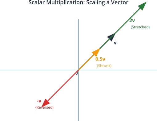
Scalar Multiplication

Scalar multiplication involves multiplying a vector by a single number (a scalar). This operation scales the vector’s magnitude. If c is a scalar and v is a vector, then:

$$c \cdot v = [c \cdot v₁, c \cdot v₂, …, c \cdot vₙ]$$

Geometrically, this operation stretches or shrinks the vector along its original direction. If c is positive, the direction remains the same. If c is negative, the vector’s direction is reversed. If $$|c| > 1$$, the vector is elongated; if $$0 < |c| < 1$$, it is contracted.

This is the fundamental mechanism for weighting in machine learning. In a neural network, the inputs to a neuron are represented by a vector. Each input is multiplied by a scalar weight, which signifies its importance. A large positive weight amplifies the input’s effect, while a weight close to zero diminishes it. The process of “learning” in a neural network is largely the process of finding the optimal set of scalar weights to apply to its input vectors. For example, in our house price predictor, the “number of bedrooms” feature might be more influential than the “year built.” This would be reflected by assigning a larger scalar weight to the “bedrooms” component of the feature vector during calculations.

The Dot Product: The Engine of Similarity and Projection

While the previous operations are foundational, the dot product (or inner product) is arguably the most important vector operation in all of machine learning. It connects the algebraic and geometric worlds and forms the computational core of countless algorithms. The dot product of two vectors u and v of the same dimension is a single scalar value, calculated by multiplying their corresponding components and summing the results:

$$u \cdot v = u₁v₁ + u₂v₂ + … + uₙvₙ = \sum_{i} uᵢvᵢ$$

This simple calculation has a profound geometric meaning. The dot product can also be expressed in terms of the vectors’ magnitudes and the angle θ between them:

$$u \cdot v = ||u|| \cdot ||v|| \cos(\theta)$$

This relationship is the key to its power. By rearranging this formula, we can understand the dot product’s two primary roles:

1. Measuring Similarity: The cos(θ) term gives us a measure of directional alignment. Cosine similarity, derived directly from the dot product, is a crucial metric in AI for determining how “alike” two vectors are, independent of their magnitudes. It is calculated as: $$\text{Cosine Similarity} = \cos(\theta) = \frac{u \cdot v}{||u|| \cdot ||v||}$$ The value ranges from -1 (pointing in opposite directions) to 1 (pointing in the same direction), with 0 indicating they are orthogonal (perpendicular). In Natural Language Processing (NLP), this is used to determine if two words or documents have similar meanings. For example, the vector for “king” would have a high cosine similarity with the vector for “queen” but a low similarity with the vector for “banana.”
2. Projecting one vector onto another: The dot product tells us the length of the projection of one vector onto another. u · v can be interpreted as the magnitude of u multiplied by the length of the component of v that lies in the direction of u. This idea of projection is central to many machine learning techniques, including Principal Component Analysis (PCA), which seeks to find the directions (vectors) onto which the data has the most variance.

In a neural network, the primary computation within a single neuron is a dot product. The neuron calculates the dot product of its input vector and its weight vector. This single number represents the total weighted sum of the inputs. A large positive dot product indicates that the inputs and weights are strongly aligned, leading to a strong activation of the neuron. This is, in essence, a pattern matching operation: the neuron “fires” when the input pattern (vector) closely matches its preferred pattern (weight vector).

graph TD
    subgraph "Input Layer"
        direction LR
        X1("x₁") ---|"w₁"| N
        X2("x₂") ---|"w₂"| N
        X3("x₃") ---|"w₃"| N
    end

    subgraph "Neuron Computation"
        N{"Σ(xᵢ * wᵢ)"} --> Z(z)
    end

    subgraph "Output "
        Z -- "Scalar Value" --> Output["Activation(z)"]:::successNode
    end

    %% Styling
    classDef inputNode fill:#9b59b6,stroke:#9b59b6,stroke-width:2px,color:#ebf5ee
    classDef processNode fill:#78a1bb,stroke:#78a1bb,stroke-width:1px,color:#283044
    classDef modelNode fill:#e74c3c,stroke:#e74c3c,stroke-width:1px,color:#ebf5ee
    classDef successNode fill:#2d7a3d,stroke:#2d7a3d,stroke-width:2px,color:#ebf5ee

    class X1,X2,X3 inputNode
    class N processNode
    class Z modelNode
    class Out_put successNode

Warning: A common mistake is to confuse the dot product, which results in a scalar, with element-wise multiplication (the Hadamard product), which results in another vector. Both are used in AI, but for very different purposes.

graph LR
    subgraph "Dot Product (u · v)"
        direction LR
        U1["u = [u₁, u₂]"] --> DP;
        V1["v = [v₁, v₂]"] --> DP{"u₁v₁ + u₂v₂"};
        DP --> Result1[("Scalar Result")];
    end

    subgraph "Hadamard Product (u ∘ v)"
        direction LR
        U2["u = [u₁, u₂]"] --> HP;
        V2["v = [v₁, v₂]"] --> HP{"[u₁v₁, u₂v₂]"};
        HP --> Result2[("Vector Result")];
    end

    %% Styling
    classDef dataNode fill:#9b59b6,stroke:#9b59b6,stroke-width:1px,color:#ebf5ee
    classDef processNode fill:#78a1bb,stroke:#78a1bb,stroke-width:1px,color:#283044
    classDef successNode fill:#2d7a3d,stroke:#2d7a3d,stroke-width:2px,color:#ebf5ee
    classDef modelNode fill:#e74c3c,stroke:#e74c3c,stroke-width:1px,color:#ebf5ee

    class U1,V1,U2,V2 dataNode;
    class DP,HP processNode;
    class Result1 successNode;
    class Result2 modelNode;

Practical Examples and Implementation

Theory provides the “what” and “why,” but practical implementation is where understanding solidifies. In this section, we will translate the mathematical concepts of vectors and their operations into executable Python code. We will heavily rely on NumPy, the fundamental package for scientific computing in Python, which provides powerful, optimized objects for handling n-dimensional arrays and matrices.

Tip: Before running these examples, ensure you have NumPy installed. You can install it via pip: pip install numpy. All examples assume you have imported the library with the standard alias: import numpy as np.

Implementing Vectors and Basic Operations in NumPy

NumPy’s core data structure, the ndarray (n-dimensional array), is the perfect tool for representing vectors. Let’s start by creating a few vectors and performing the basic operations we’ve discussed.

Creating Vectors

A vector is simply a 1D NumPy array.

import numpy as np

# Create a 2D vector representing a point (2, 3)
v_2d = np.array([2, 3])

# Create a 4D vector representing our house example
# [square footage, bedrooms, bathrooms, year built]
# We'll scale the features for this example to keep numbers manageable
house_vector = np.array([1.5, 3.0, 2.0, 2.005]) 

print(f"A 2D vector: {v_2d}")
print(f"A 4D house feature vector: {house_vector}")

Vector Addition and Subtraction

Let’s imagine we have two users in a movie recommendation system, represented by their ratings for three genres: Action, Comedy, and Sci-Fi.

import numpy as np

# User A's preference vector [Action, Comedy, Sci-Fi]
user_a_prefs = np.array([5, 2, 4])

# User B's preference vector
user_b_prefs = np.array([3, 5, 1])

# To find their combined interest profile, we add their vectors
combined_prefs = user_a_prefs + user_b_prefs
print(f"Combined preferences: {combined_prefs}")

# To find how different their tastes are, we can subtract them
# This creates a "difference" vector
taste_difference = user_a_prefs - user_b_prefs
print(f"Taste difference (A - B): {taste_difference}")

The combined_prefs vector [8, 7, 5] shows a strong aggregate interest in Action. The taste_difference vector [2, -3, 3] shows that User A likes Action and Sci-Fi more than User B, but User B has a much stronger preference for Comedy.

Scalar Multiplication

Now, let’s say we want to apply a “weight” to a feature vector. In our house price example, perhaps the square footage is twice as important as the other features in a simplified model. We can use scalar multiplication to reflect this.

import numpy as np

# A simple 2D feature vector [size, location_score]
house_features = np.array([1200, 8]) # 1200 sq ft, location score of 8/10

# Let's say we have a simple pricing model where the final price is a scaled
# version of this feature vector. The scaling factor is our scalar.
price_scalar = 250.5

# Calculate the weighted feature values
weighted_features = price_scalar * house_features
print(f"Original features: {house_features}")
print(f"Weighted features: {weighted_features}")

This operation scales both components, showing how a single factor can uniformly increase the influence of all features. In more complex models, we would use a vector of different scalars (weights) and perform a dot product.

The Dot Product in Action: A Simple Prediction Model

The dot product is the workhorse of prediction. Let’s build a very simple linear model to predict a student’s final exam score based on hours studied, previous test scores, and attendance.

The model is: $$\text{Predicted Score} = (w₁ \cdot \text{hours}) + (w₂ \cdot \text{prev_score}) + (w₃ \cdot \text{attendance})$$

This is a dot product!

import numpy as np

# Feature vector for a student:
# [hours_studied, avg_previous_score, attendance_percentage]
student_features = np.array([15.5, 88, 0.95])

# Weight vector determined by our "trained" model.
# These weights signify the importance of each feature.
# Here, previous score is most important, followed by hours studied.
weights = np.array([2.5, 1.0, 10.0])

# Calculate the predicted score using the dot product
# NumPy has a dedicated function: np.dot()
predicted_score = np.dot(student_features, weights)

print(f"Student Feature Vector: {student_features}")
print(f"Model Weight Vector: {weights}")
print(f"Predicted Final Exam Score: {predicted_score:.2f}")

# You can also use the @ operator for dot products in Python 3.5+
predicted_score_alt = student_features @ weights
print(f"Predicted Score (using @): {predicted_score_alt:.2f}")

This single dot product operation elegantly combines all features with their respective importances to produce a single, meaningful prediction. This is precisely what happens inside every neuron of a neural network, but on a much larger scale.

Visualization and Computational Exercises

Visualizing vectors helps build intuition. Let’s use Matplotlib to see our operations.

Visualizing Vector Addition

import numpy as np
import matplotlib.pyplot as plt

# Define two vectors
u = np.array([2, 5])
v = np.array([4, 1])
sum_uv = u + v

# Plotting setup
plt.figure(figsize=(8, 8))
ax = plt.gca()
ax.quiver(0, 0, u[0], u[1], angles='xy', scale_units='xy', scale=1, color='r', label='u = [2, 5]')
ax.quiver(u[0], u[1], v[0], v[1], angles='xy', scale_units='xy', scale=1, color='b', label='v = [4, 1]')
ax.quiver(0, 0, sum_uv[0], sum_uv[1], angles='xy', scale_units='xy', scale=1, color='g', label='u + v = [6, 6]')

# Set plot limits and labels
ax.set_xlim([0, 8])
ax.set_ylim([0, 8])
plt.title('Geometric Interpretation of Vector Addition')
plt.xlabel('X-axis')
plt.ylabel('Y-axis')
plt.grid()
plt.legend()
plt.show()

This code generates a plot that visually confirms the parallelogram rule, showing how adding v to the tip of u results in the sum vector u + v.

Computational Exercise: Cosine Similarity

Objective: Write a Python function to calculate the cosine similarity between two vectors. Use it to determine which of two documents is more similar to a query document.

Problem:

• Query Document Vector: [1, 1, 0, 1] (Represents presence of words: ‘AI’, ‘learning’, ‘data’, ‘model’)
• Document A Vector: [1, 1, 0, 1] (Represents: ‘AI’, ‘learning’, ‘data’, ‘model’)
• Document B Vector: [0, 1, 1, 0] (Represents: ‘python’, ‘learning’, ‘data’, ‘science’)

Manual Calculation First:

1. Dot Product (Query · A): $$(1 \cdot 1) + (1 \cdot 1) + (0 \cdot 0) + (1 \cdot 1) = 3$$
2. Magnitude (||Query||): $$\sqrt{1² + 1² + 0² + 1²} = \sqrt{3}$$
3. Magnitude (||A||): $$sqrt(1²+1²+0²+1²) = sqrt(3)$$
4. Cosine Similarity (Query, A): $$3 / (\sqrt{3} \cdot \sqrt{3}) = 3 / 3 = 1.0$$ (Perfect match)
5. Dot Product (Query · B): $$(1 \cdot 0) + (1 \cdot 1) + (0 \cdot 1) + (1 \cdot 0) = 1$$
6. Magnitude (||B||): $$\sqrt{0² + 1² + 1² + 0²} = \sqrt{2}$$
7. Cosine Similarity (Query, B): $$1 / (\sqrt{3} \cdot \sqrt{2}) = 1 / \sqrt{6} \approx 0.408$$

Implementation:

import numpy as np

def cosine_similarity(vec1, vec2):
    """Calculates the cosine similarity between two non-zero vectors."""
    dot_product = np.dot(vec1, vec2)
    norm_vec1 = np.linalg.norm(vec1)
    norm_vec2 = np.linalg.norm(vec2)
    
    # Avoid division by zero
    if norm_vec1 == 0 or norm_vec2 == 0:
        return 0.0
        
    return dot_product / (norm_vec1 * norm_vec2)

# Document vectors
query_doc = np.array([1, 1, 0, 1])
doc_a = np.array([1, 1, 0, 1])
doc_b = np.array([0, 1, 1, 0])

# Calculate similarities
sim_a = cosine_similarity(query_doc, doc_a)
sim_b = cosine_similarity(query_doc, doc_b)

print(f"Similarity between Query and Document A: {sim_a:.4f}")
print(f"Similarity between Query and Document B: {sim_b:.4f}")

if sim_a > sim_b:
    print("Conclusion: Document A is more similar to the query.")
else:
    print("Conclusion: Document B is more similar to the query.")

This practical example demonstrates how the dot product, combined with the concept of the norm, provides a powerful and widely used mechanism for information retrieval and recommendation systems.

graph TD
    A[Start: Two Vectors u, v] --> B{Calculate Dot Product: u · v};
    A --> C{"Calculate Magnitude of u: ||u||"};
    A --> D{"Calculate Magnitude of v: ||v||"};

    subgraph "Combine Results"
        B --> E;
        C --> E;
        D --> E{"(u · v) / (||u|| * ||v||)"};
    end

    E --> F[Result: Cosine Similarity Score];
    F --> G{Score = 1?};
    F --> H{Score = 0?};
    F --> I{Score = -1?};

    G -- "Same Direction" --> J((Perfect Similarity));
    H -- "Orthogonal (90°)" --> K((No Similarity));
    I -- "Opposite Directions" --> L((Perfect Dissimilarity));

    %% Styling
    classDef startNode fill:#283044,stroke:#283044,stroke-width:2px,color:#ebf5ee
    classDef processNode fill:#78a1bb,stroke:#78a1bb,stroke-width:1px,color:#283044
    classDef dataNode fill:#9b59b6,stroke:#9b59b6,stroke-width:1px,color:#ebf5ee
    classDef decisionNode fill:#f39c12,stroke:#f39c12,stroke-width:1px,color:#283044
    classDef successNode fill:#2d7a3d,stroke:#2d7a3d,stroke-width:2px,color:#ebf5ee
    classDef warningNode fill:#f1c40f,stroke:#f1c40f,stroke-width:1px,color:#283044
    classDef errorNode fill:#d63031,stroke:#d63031,stroke-width:1px,color:#ebf5ee

    class A startNode;
    class B,C,D,E processNode;
    class F dataNode;
    class G,H,I decisionNode;
    class J successNode;
    class K warningNode;
    class L errorNode;

Industry Applications and Case Studies

The abstract concepts of vector operations translate into billions of dollars of business value across numerous industries. Their implementation is the engine behind personalization, automation, and data-driven decision-making.

1. E-commerce and Media Recommendation Engines (Netflix, Amazon, Spotify):

• Application: At the heart of platforms like Netflix and Spotify are recommendation systems that predict what a user might like next. Each user and each item (movie, song, product) is represented as a high-dimensional vector in a shared “embedding space.”
• Technical Implementation: The components of these vectors, known as embeddings, are learned automatically by machine learning models (often using techniques like matrix factorization). A user’s vector is positioned based on their historical behavior. An item’s vector is positioned based on its characteristics and how other users have interacted with it. To generate recommendations, the system calculates the dot product or cosine similarity between a user’s vector and the vectors of millions of items. Items with the highest similarity scores are then recommended.
• Business Impact: This hyper-personalization is directly responsible for increasing user engagement, retention, and sales. Netflix has stated that its recommendation system saves it over $1 billion per year by reducing subscriber churn.

2. Semantic Search and Large Language Models (Google, OpenAI):

• Application: Modern search engines and LLMs like GPT-4 go beyond simple keyword matching. They understand the meaning or semantic intent behind a query.
• Technical Implementation: Every word, sentence, or document is mapped to a vector embedding. The query “top AI research papers from last year” is converted into a vector. The system then searches a massive database of document vectors to find those with the highest cosine similarity to the query vector. This allows it to find relevant documents that may not even contain the exact keywords but are semantically related (e.g., an article about “breakthroughs in machine learning in 2024”). The dot product is used trillions of times a day to power these searches.
• Business Impact: The ability to understand intent provides vastly more relevant results, which is the core business value of a search engine. For LLMs, vector similarity is fundamental to retrieval-augmented generation (RAG), where the model retrieves relevant information before generating an answer.

3. Computer Vision for Autonomous Vehicles (Tesla, Waymo):

• Application: Autonomous systems must identify and track objects like pedestrians, other cars, and traffic signs in real-time from sensor data (e.g., cameras, LiDAR).
• Technical Implementation: An object detected in an image is represented by a feature vector extracted by a deep convolutional neural network (CNN). This vector encodes information about the object’s appearance. To track the object across consecutive video frames, the system compares the feature vector of the object in the current frame to potential object vectors in the next frame using vector subtraction to find the smallest “difference” or distance (often the Euclidean distance, which is derived from the dot product of the difference vector with itself).
• Business Impact: Reliable and fast object tracking is a critical safety component for autonomous driving. The efficiency of vectorized operations on GPUs is what makes real-time performance possible, enabling a core function of the multi-trillion-dollar autonomous vehicle market.

Best Practices and Common Pitfalls

Mastering vector operations in practice involves more than just knowing the formulas. It requires adopting professional workflows and being aware of common errors that can compromise performance and accuracy.

1. Embrace Vectorization for Performance:

• Best Practice: Always prefer vectorized operations over explicit loops in Python. NumPy, TensorFlow, and PyTorch are built on highly optimized, low-level C++ and Fortran code. A single vectorized operation like C = A + B in NumPy can be orders of magnitude faster than iterating through the elements in a Python for loop. This is because the loop is executed in compiled code, avoids the overhead of Python’s interpreter for each element, and can leverage modern CPU/GPU hardware for parallel processing.
• Common Pitfall: Writing Python loops to perform element-wise arithmetic on large arrays. This is a classic sign of a beginner and leads to extremely inefficient, slow code that will not scale to production datasets.

2. Maintain Dimensionality Awareness:

• Best Practice: Always be certain of the shapes (dimensions) of your vectors and matrices. Use the .shape attribute in NumPy frequently during development and debugging. Before performing an operation like a dot product, mentally (or with an assertion) confirm that the inner dimensions align. For np.dot(A, B), the number of columns in A must equal the number of rows in B.
• Common Pitfall: Encountering ValueError: shapes (m,n) and (p,q) not aligned at runtime. This is one of the most common errors in machine learning code. It almost always stems from a misunderstanding of the data’s shape or a mistake in a preceding transformation step. Proactive shape checking can prevent these errors.

3. The Importance of Feature Scaling:

• Best Practice: Before feeding feature vectors into many ML algorithms (especially those that rely on distance calculations, like k-NN, or gradient-based optimization, like neural networks), scale your features. Common techniques include Standardization (scaling to zero mean and unit variance) and Normalization (scaling to a range, typically [0, 1]).
• Common Pitfall: Using raw, unscaled features. If one feature (e.g., house price in dollars) has a much larger magnitude than another (e.g., number of bedrooms), the high-magnitude feature will dominate calculations like the dot product and Euclidean distance. This can cause optimization algorithms to struggle to converge and lead to a model that is biased towards the feature with the largest scale, not the one that is most informative.

4. Distinguish Dot Product from Element-wise Multiplication:

• Best Practice: Be deliberate in your choice of multiplication. Use np.dot() or the @ operator for the true dot product (linear algebraic matrix multiplication). Use * for element-wise multiplication (the Hadamard product).
• Common Pitfall: Using * when you intend to perform a dot product. For two vectors, this will work by coincidence if they are 1D arrays, but it will produce incorrect results for matrices and is conceptually wrong. This error can be subtle and hard to debug as it may not raise an exception but will lead to incorrect model outputs.

Warning: Floating-point precision can be an issue in large-scale computations. While usually not a problem for basic operations, be aware that comparing two floating-point numbers for exact equality (a == b) is often a mistake. It’s better to check if they are close within a small tolerance: np.isclose(a, b).

Hands-on Exercises

These exercises are designed to reinforce the concepts from the chapter, progressing from basic implementation to practical application.

Exercise 1: Vector Manipulation and Visualization

• Objective: Practice basic vector creation, arithmetic, and plotting.
• Tasks:
  1. Create two 2D vectors, a = [8, 2] and b = [-3, 4].
  2. Calculate the following: c = a + b, d = a - b, and e = 2.5 * a.
  3. Calculate the magnitude (L2 norm) of all five vectors (a, b, c, d, e).
  4. Using Matplotlib, create a single plot that visualizes vectors a, b, and c originating from the origin.
• Success Criteria: Your code should run without errors, produce the correct numerical results for the new vectors and their magnitudes, and generate a clear plot showing the three vectors.

Exercise 2: Building a Simple Content Filter

• Objective: Use the dot product to create a basic filter for content based on weighted features.
• Scenario: You are building a system to flag potentially inappropriate online comments. You have a simple model that uses a weight vector to score comments based on a feature vector.
• Tasks:
  1. Define a weights vector: w = [0.8, 0.5, 0.2]. These correspond to the features: ‘profanity_count’, ‘all_caps_word_ratio’, ‘exclamation_mark_count’.
  2. You receive three new comments with the following feature vectors:
     • comment1 = [5, 0.1, 1] (High profanity, low caps, few exclamations)
     • comment2 = [0, 0.9, 15] (No profanity, mostly caps, many exclamations)
     • comment3 = [1, 0.2, 2] (Low profanity, low caps, some exclamations)
  3. For each comment, calculate its “risk score” by taking the dot product of its feature vector and the weight vector.
  4. Set a threshold of 4.0. Any comment with a score above this threshold should be flagged. Print which comments are flagged.
• Success Criteria: The program should correctly calculate the risk score for each comment and print a message indicating whether each one is flagged based on the threshold.

Exercise 3: Team Activity – Finding the Most Similar User

• Objective: Apply cosine similarity to solve a practical recommendation problem.
• Scenario: You are given a target user and a small dataset of other users. Your goal is to find which user in the dataset has the most similar tastes to the target user. Tastes are represented by vectors of movie genre ratings.
• Tasks:
  1. Define the target_user vector: [5, 4, 1, 0, 5] (ratings for Sci-Fi, Fantasy, Romance, Horror, Action).
  2. Define a list or dictionary of other users and their rating vectors:
     • user1 = [4, 5, 2, 1, 4]
     • user2 = [1, 0, 5, 5, 0]
     • user3 = [5, 4, 1, 1, 5]
  3. Write a program that iterates through the other users, calculates the cosine similarity between each user and the target_user, and keeps track of the user with the highest similarity score.
  4. Print the name of the most similar user and their similarity score.
• Success Criteria: The program should correctly identify user3 as the most similar, as their vector has the most similar direction to the target user’s vector, and output the corresponding similarity score.

Tools and Technologies

The concepts in this chapter are universal, but their practical implementation relies on a specific set of tools that are standard in the AI/ML industry.

• Python (3.9+): The undisputed dominant programming language for AI development. Its clear syntax, extensive libraries, and strong community support make it the ideal choice. All examples in this book use modern Python.
• NumPy (Numerical Python): The foundational library for numerical computing in Python. It provides the ndarray object, which is a highly efficient, multi-dimensional array, and a vast collection of mathematical functions to operate on these arrays. It is the bedrock upon which most other scientific Python libraries are built.
  • Installation: pip install numpy
  • Key Feature: Its ability to perform fast, vectorized operations is critical for performance.
• SciPy (Scientific Python): Built on top of NumPy, SciPy provides a larger collection of more specialized scientific algorithms. For vector operations, its scipy.linalg module offers more advanced linear algebra capabilities than NumPy, and scipy.spatial.distance contains optimized functions for computing distances, including cosine distance.
  • Installation: pip install scipy
  • When to use: When you need more advanced linear algebra functions or specialized distance metrics.
• Matplotlib & Seaborn: These are the primary libraries for data visualization in Python.
  • Matplotlib: A powerful, low-level library that gives you fine-grained control over every aspect of a plot. Excellent for creating custom visualizations like the vector plots in this chapter. (pip install matplotlib)
  • Seaborn: A high-level library built on Matplotlib that provides a more aesthetically pleasing and statistically oriented interface for common plot types.
  • Integration: They integrate seamlessly with NumPy, allowing you to directly plot data from ndarray objects.
• Jupyter Notebooks / JupyterLab: An interactive development environment that allows you to write and execute code in cells, interspersing it with text, equations, and visualizations. It is an invaluable tool for exploratory data analysis, prototyping models, and creating educational materials like this chapter.

Summary

This chapter established the critical role of vectors as the fundamental language of data in AI and machine learning. We moved from abstract theory to practical, hands-on implementation.

• Core Concepts: We defined vectors as points in a multi-dimensional feature space, possessing both magnitude and direction.
• Fundamental Operations: We explored the element-wise operations of vector addition, subtraction, and scalar multiplication, understanding their geometric interpretations of combination, difference, and scaling.
• The Dot Product: We identified the dot product as the most crucial operation, serving as the engine for calculating weighted sums in neural networks and for measuring directional alignment via cosine similarity.
• Practical Implementation: We translated these mathematical concepts into efficient Python code using the NumPy library, emphasizing the performance benefits of vectorization over manual loops.
• Real-World Relevance: We connected these foundational operations to high-value industry applications, including recommendation engines, semantic search, and computer vision.

The skills gained in this chapter are not merely academic. Your ability to represent problems in terms of vectors and manipulate them using these core operations is the first and most important step in designing, building, and debugging any machine learning model.

Further Reading and Resources

1. 3Blue1Brown – Essence of Linear Algebra: An outstanding video series that provides deep visual intuitions for linear algebra concepts, including vectors, dot products, and more. Essential viewing for any aspiring AI engineer. https://www.youtube.com/playlist?list=PLZHQObOWTQDPD3MizzM2xVFitgF8hE_ab
2. NumPy Official Documentation: The definitive source for all NumPy functions and features. The “NumPy: the absolute basics for beginners” tutorial is an excellent starting point. https://numpy.org/doc/stable/user/absolute_beginners.html
3. Deep Learning by Ian Goodfellow, Yoshua Bengio, and Aaron Courville: Chapter 2, “Linear Algebra,” provides a concise and rigorous overview of the mathematical concepts essential for deep learning. Available online for free. https://www.deeplearningbook.org/
4. “Introduction to Linear Algebra” by Gilbert Strang: A classic and highly respected textbook on linear algebra from an MIT professor. It provides a comprehensive and accessible treatment of the subject.
5. SciPy Lecture Notes: A collection of tutorials on the scientific Python ecosystem, with excellent sections on linear algebra and optimization. https://lectures.scientific-python.org/

Glossary of Terms

• Vector: An ordered list of numbers that represents a point in a multi-dimensional space. It has both magnitude and direction.
• Scalar: A single numerical quantity, as opposed to a vector or matrix.
• Component: An individual number within a vector. Also known as an element.
• Dimensionality: The number of components in a vector, corresponding to the number of axes or features in its space.
• Magnitude (Norm): The length or size of a vector. The most common is the L2 norm (Euclidean norm).
• Vector Addition: An element-wise operation that combines two vectors of the same dimension into a resultant vector.
• Scalar Multiplication: An operation that multiplies a vector by a scalar, scaling its magnitude.
• Dot Product (Inner Product): An operation that takes two vectors and returns a single scalar. It is calculated as the sum of the products of their corresponding components. Crucial for measuring similarity and projection.
• Cosine Similarity: A metric derived from the dot product used to measure the directional similarity of two vectors, independent of their magnitudes. Values range from -1 to 1.
• Vectorization: The practice of using optimized library functions (like those in NumPy) to perform operations on entire arrays at once, rather than iterating through elements in a loop.