
Chapter 13: Probability Theory: Basic Concepts and Distributions
Chapter Objectives
Upon completing this chapter, students will be able to:
- Understand the foundational axioms of probability theory and their role in quantifying uncertainty in AI systems.
- Analyze and differentiate between discrete and continuous random variables, and compute their essential properties such as expected value, variance, and standard deviation.
- Implement common probability distributions (e.g., Bernoulli, Binomial, Normal, Poisson) using Python libraries like NumPy and SciPy to model real-world phenomena.
- Apply Bayes’ theorem to solve problems involving conditional probability, forming the basis for understanding fundamental machine learning algorithms like Naive Bayes.
- Design and interpret visualizations of probability distributions and statistical data using Matplotlib and Seaborn to gain insights and communicate findings effectively.
- Evaluate the suitability of different probability distributions for modeling specific types of data and uncertainty in AI engineering contexts.
Introduction
In the landscape of Artificial Intelligence and Machine Learning, few disciplines are as fundamental as probability theory. While deterministic algorithms have their place, the real world is fraught with randomness, incomplete information, and inherent uncertainty. From predicting stock market fluctuations to understanding the nuances of human language, the ability to model and reason under uncertainty is what elevates a simple algorithm to an intelligent system. Probability theory provides the mathematical language for this endeavor. It is the bedrock upon which we build models that can learn from data, make predictions about the future, and quantify their own confidence.
This chapter serves as a formal introduction to the principles of probability that are indispensable for any AI engineer. We will move beyond a superficial understanding to build a robust theoretical and practical foundation. You will learn how abstract concepts like sample spaces and axioms translate into powerful tools for data analysis and model building. We will explore random variables and the key probability distributions that serve as the building blocks for some of the most sophisticated models in machine learning, from generative models that can create realistic images to Bayesian neural networks that know when they are uncertain. By the end of this chapter, you will not only grasp the core mathematics but also be equipped to implement these concepts in Python, turning theoretical knowledge into a practical skill set essential for a career in modern AI development.
Technical Background
The journey into machine learning is, in many respects, a journey into applied probability. The goal of most learning algorithms is to distill patterns from data, and these patterns are often best described through a probabilistic lens. This section lays the groundwork by introducing the core concepts of probability theory, establishing the mathematical formalism required to build and understand complex AI models.
The Foundations of Probability
At its core, probability theory is a mathematical framework for quantifying uncertainty. To do so rigorously, we must first define the basic elements of a probabilistic model.
| Concept | Definition | Example (Rolling a 6-Sided Die) |
|---|---|---|
| Sample Space (Ω) | The set of all possible outcomes of an experiment. | Ω = {1, 2, 3, 4, 5, 6} |
| Event (A) | A subset of the sample space Ω. | Event A: “Rolling an even number” A = {2, 4, 6} |
| Axiom 1: Non-negativity | The probability of any event is non-negative. | P(A) ≥ 0. The probability of rolling an even number is 3/6 = 0.5, which is ≥ 0. |
| Axiom 2: Normalization | The probability of the entire sample space is 1. | P(Ω) = 1. The probability of rolling any number from 1 to 6 is 1. |
| Axiom 3: Additivity | For mutually exclusive events A and B, the probability of A or B occurring is the sum of their probabilities. | Let B = {1}. A and B are disjoint. P(A ∪ B) = P(A) + P(B) = 3/6 + 1/6 = 4/6. |
Sample Spaces, Events, and Axioms
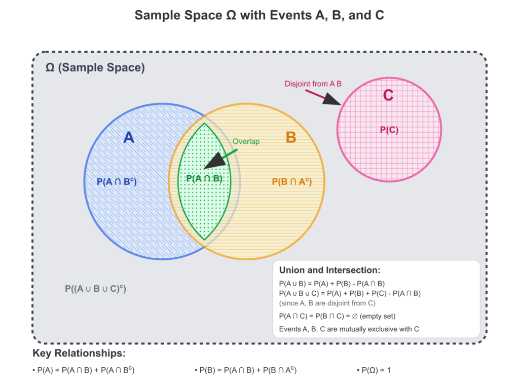
The starting point for any probabilistic analysis is the experiment, which is any procedure that can be infinitely repeated and has a well-defined set of possible outcomes. The set of all possible outcomes of an experiment is called the sample space, typically denoted by \(\Omega\) (Omega). For example, if our experiment is a single coin toss, the sample space is \(\Omega = {Heads, Tails}\). If we are rolling a standard six-sided die, the sample space is \(\Omega = {1, 2, 3, 4, 5, 6}\).
An event, denoted by a capital letter like \(A\), is any subset of the sample space \(\Omega\). An event is said to have occurred if the outcome of the experiment is an element of that set. In the die-rolling experiment, the event “rolling an even number” would be the set \(A = {2, 4, 6}\). The event “rolling a number greater than 4” would be \(B = {5, 6}\).
The entire field of probability is built upon three simple but powerful axioms, formulated by the Russian mathematician Andrey Kolmogorov in the 1930s. These axioms define a function \(P\), the probability measure, which assigns a real number to every event \(A\).
1. Non-negativity: The probability of any event is non-negative.P(A)ge0quadtextforanyeventAsubseteqOmega
\[P(A) \ge 0 \quad \text{for any event } A \subseteq \Omega\]
2. Normalization: The probability of the entire sample space is 1. This means that at least one of the possible outcomes must occur. \[P(\Omega) = 1\]
3. Additivity for Mutually Exclusive Events: If two events \(A\) and \(B\) are mutually exclusive (or disjoint), meaning they have no outcomes in common (\(A \cap B = \emptyset\)), then the probability that either \(A\) or \(B\) occurs is the sum of their individual probabilities. \[P(A \cup B) = P(A) + P(B) \quad \text{if } A \cap B = \emptyset\] This extends to any countable sequence of mutually exclusive events.
From these three axioms, all other properties of probability can be derived. For instance, we can prove that the probability of the empty set (an impossible event) is \(P(\emptyset) = 0\), and for any event \(A\), its probability is bounded by \(0 \le P(A) \le 1\).
Conditional Probability and Independence
Often, we are interested in the probability of an event given that another event has already occurred. This is known as conditional probability. The conditional probability of event \(A\) occurring given that event \(B\) has occurred is defined as:\[P(A|B) = \frac{P(A \cap B)}{P(B)}, \quad \text{provided } P(B) > 0\]
Here, \(P(A \cap B)\) is the probability of both \(A\) and \(B\) occurring, also known as the joint probability. The formula essentially re-scales the probability of the joint event by the new, reduced sample space defined by event \(B\). For example, in our die-rolling experiment, what is the probability of rolling a 2 (\(A={2}\)) given that we know an even number was rolled (\(B={2, 4, 6}\))? The intersection is \(A \cap B = {2}\). Assuming a fair die, \(P(A \cap B) = P({2}) = 1/6\) and \(P(B) = P({2, 4, 6}) = 3/6 = 1/2\). Therefore, \(P(A|B) = \frac{1/6}{1/2} = 1/3\). This makes intuitive sense: given that the outcome is one of the three even numbers, the chance of it being a 2 is one in three.
A related and crucial concept is independence. Two events \(A\) and \(B\) are said to be independent if the occurrence of one does not affect the probability of the other. Mathematically, this means: \[P(A∣B)=P(A)\]
If this holds, it follows from the definition of conditional probability that for independent events:P(AcapB)=P(A)P(B)
This is a fundamental relationship used throughout machine learning. For instance, the “naive” assumption in the Naive Bayes classifier is that all features are conditionally independent of each other given the class label. While this assumption is often violated in practice, it dramatically simplifies the model and often yields surprisingly good results.
Warning: Do not confuse mutually exclusive events with independent events. If two events \(A\) and \(B\) with non-zero probabilities are mutually exclusive, they cannot be independent. The occurrence of \(A\) (\(A \cap B = \emptyset\)) means \(B\) cannot occur, so \(P(B|A) = 0 \neq P(B)\).
Bayes’ Theorem: The Engine of Inference
One of the most important results derived from conditional probability is Bayes’ theorem. It provides a way to update our beliefs about a hypothesis in light of new evidence. By rearranging the definition of conditional probability, we know \(P(A \cap B) = P(A|B)P(B)\) and \(P(B \cap A) = P(B|A)P(A)\). Since \(P(A \cap B) = P(B \cap A)\), we can set these equal and solve for \[P(A|B) = \frac{P(B|A)P(A)}{P(B)}\]
This is Bayes’ theorem. In the context of machine learning, we often frame it using different terminology:\[P(\text{hypothesis}|\text{evidence}) = \frac{P(\text{evidence}|\text{hypothesis})P(\text{hypothesis})}{P(\text{evidence})}\]
Let’s break down the terms:
- \(P(\text{hypothesis}|\text{evidence})\) is the posterior probability: the probability of our hypothesis after observing the evidence. This is what we typically want to compute.
- \(P(\text{evidence}|\text{hypothesis})\) is the likelihood: the probability of observing the evidence given that our hypothesis is true. This is often calculated from our model.
- \(P(\text{hypothesis})\) is the prior probability: our initial belief in the hypothesis before seeing any evidence.
- \(P(\text{evidence})\) is the marginal likelihood or evidence: the total probability of observing the evidence, summed over all possible hypotheses. It acts as a normalization constant.
Bayes’ theorem is the foundation of Bayesian statistics and a vast array of machine learning models. It allows us to move from a prior belief to an updated posterior belief as we gather data, formalizing the process of learning from experience.
        graph TD
            A[("<b>Prior Belief</b><br><i>P(Hypothesis)</i><br>Initial belief before evidence")]
            B[("<b>Likelihood</b><br><i>P(Evidence | Hypothesis)</i><br>How well the hypothesis explains the data")]
            C{{"<b>Bayes' Theorem</b><br>Combine Prior and Likelihood"}}
            D[("<b>Posterior Belief</b><br><i>P(Hypothesis | Evidence)</i><br>Updated belief after seeing evidence")]
            E(Data / Evidence)

            A --> C
            B --> C
            E --> B

            C --> D

            classDef startNode fill:#283044,stroke:#283044,stroke-width:2px,color:#ebf5ee
            classDef processNode fill:#78a1bb,stroke:#78a1bb,stroke-width:1px,color:#283044
            classDef decisionNode fill:#f39c12,stroke:#f39c12,stroke-width:1px,color:#283044
            classDef endNode fill:#2d7a3d,stroke:#2d7a3d,stroke-width:2px,color:#ebf5ee
            classDef dataNode fill:#9b59b6,stroke:#9b59b6,stroke-width:1px,color:#ebf5ee

            class A,B startNode
            class C decisionNode
            class D endNode
            class E dataNode
Random Variables and Their Properties
While events are useful, it is often more convenient to work with numerical representations of the outcomes of an experiment. This is the role of a random variable. A random variable, typically denoted by a capital letter like \(X\), is a function that maps outcomes from the sample space \(\Omega\) to real numbers.
For example, in an experiment of tossing two coins, the sample space is \(\Omega = {HH, HT, TH, TT}\). We could define a random variable \(X\) to be the number of heads observed. Then \(X\) would map the outcomes as follows: \(X(HH) = 2\), \(X(HT) = 1\), \(X(TH) = 1\), and \(X(TT) = 0\). The set of possible values that \(X\) can take is \({0, 1, 2}\).
Random variables are broadly classified into two types: discrete and continuous.
Discrete Random Variables
A discrete random variable is one that can take on a finite or countably infinite number of distinct values. The variable \(X\) representing the number of heads in two coin tosses is discrete.
The probabilistic behavior of a discrete random variable is described by its Probability Mass Function (PMF), denoted \(p(x)\). The PMF gives the probability that the random variable \(X\) is exactly equal to some value \(x\):\[p(x)=P(X=x)\]
For a valid PMF, two conditions must be met: \(p(x) \ge 0\) for all \(x\), and \(\sum_x p(x) = 1\), where the sum is over all possible values of \(X\).
Continuous Random Variables
A continuous random variable is one that can take on any value within a given range or interval. Examples include the height of a person, the temperature of a room, or the time it takes for a server to respond to a request.
For a continuous random variable, the probability of it taking on any single specific value is zero, i.e., \(P(X=x) = 0\). This is because there are infinitely many possible values in any interval. Instead, we talk about the probability of \(X\) falling within a certain range. This is described by the Probability Density Function (PDF), denoted \(f(x)\). The PDF is not a probability itself, but its integral over a range gives the probability for that range:\[P(a \le X \le b) = \int_a^b f(x) ,dx\]
For a valid PDF, two conditions must be met: \(f(x) \ge 0\) for all \(x\), and \(\int_{-\infty}^{\infty} f(x) ,dx = 1\). The value of \(f(x)\) can be thought of as the “density” of probability around the point \(x\).
Comparison of Random Variables
| Feature | Discrete Random Variable | Continuous Random Variable |
|---|---|---|
| Values | Finite or countably infinite distinct values. | Uncountably infinite values within a range. |
| Examples | Number of heads in 3 coin flips, number of defective items, die roll result. | Height of a person, temperature, time to complete a task. |
| Probability Function | Probability Mass Function (PMF): p(x) = P(X=x) | Probability Density Function (PDF): f(x) |
| Probability Interpretation | PMF gives the probability of a specific outcome. | Probability is the area under the PDF curve over an interval: P(a ≤ X ≤ b). |
| Key Condition | The sum of all probabilities is 1: Σ p(x) = 1 | The total area under the PDF curve is 1: ∫ f(x)dx = 1 |
| Expected Value E[X] | Σ x * p(x) | ∫ x * f(x) dx |
Expected Value and Variance
Two of the most important properties of any random variable are its expected value and variance.
The expected value (or mean), denoted \(E[X]\) or \(\mu\), is the long-run average value of the random variable over many repetitions of the experiment. It is a weighted average of the possible values, where the weights are the probabilities (or densities).
- For a discrete random variable \(X\):\[E[X]=\sum_x x \cdot p(x)\]
- For a continuous random variable \(X\):\[\int_{-\infty}^{\infty} x \cdot f(x) ,dx\]
The variance, denoted \(Var(X)\) or \(\sigma^2\), measures the spread or dispersion of the random variable’s values around its mean. A low variance indicates that the values tend to be close to the mean, while a high variance indicates that they are spread out. The variance is defined as the expected value of the squared deviation from the mean:\[Var(X)=E[(X−E[X])2]=E[(X−\sigma)^2]\]
A more convenient computational formula is \(Var(X) = E[X^2] – (E[X])^2\). The standard deviation, \(\sigma\), is simply the square root of the variance, \(\sigma = \sqrt{Var(X)}\). It is often preferred because it is in the same units as the random variable itself.
Common Probability Distributions in AI
In practice, we rarely derive PMFs or PDFs from scratch. Instead, we use a family of well-understood probability distributions that serve as models for various types of real-world processes. Choosing the correct distribution to model your data is a critical step in AI engineering.
Common Probability Distributions in AI
| Distribution | Type | Parameters | Description & Use Case |
|---|---|---|---|
| Bernoulli | Discrete | p (probability of success) | Models a single trial with two outcomes (e.g., success/failure, click/no-click). Foundation for binary classification. |
| Binomial | Discrete | n (trials), p (success prob.) | Models the number of successes in ‘n’ independent Bernoulli trials. E.g., number of fraudulent transactions in a batch. |
| Poisson | Discrete | λ (average rate) | Models the number of events in a fixed interval of time/space. E.g., number of visitors to a website per hour. |
| Uniform | Continuous | a (min), b (max) | All outcomes in a range [a, b] are equally likely. Used for non-informative priors or weight initialization. |
| Normal (Gaussian) | Continuous | μ (mean), σ² (variance) | The “bell curve”. Models natural phenomena, noise in data, and sums of random variables (due to CLT). Ubiquitous in ML. |
| Exponential | Continuous | λ (rate) or β=1/λ (scale) | Models the time between events in a Poisson process. Used in survival analysis and reliability engineering (e.g., component lifetime). |
Discrete Distributions
- Bernoulli Distribution: This is the simplest distribution, modeling a single trial with two possible outcomes (e.g., success/failure, heads/tails, 1/0). It is governed by a single parameter \(p\), the probability of success. If \(X \sim \text{Bernoulli}(p)\), then \(P(X=1) = p\) and \(P(X=0) = 1-p\). This is the building block for many other distributions and is fundamental to binary classification tasks in machine learning.
- Binomial Distribution: This describes the number of successes in a fixed number, \(n\), of independent and identical Bernoulli trials, each with a probability of success \(p\). If \(X \sim \text{Binomial}(n, p)\), its PMF is given by:\[P(X = k) = \left(\begin{array}{c} n \ k \end{array}\right) p^k (1-p)^{n-k}\] where \[\left(\begin{array}{c} n \ k \end{array}\right) = \frac{n!}{k!(n-k)!}\]is the binomial coefficient. It is used to model phenomena like the number of fraudulent transactions in a batch of 100, or the number of defective items in a production run.
- Poisson Distribution: This models the number of events occurring in a fixed interval of time or space, given a constant mean rate \(\lambda\) at which the events occur. If \(X \sim \text{Poisson}(\lambda)\), its PMF is:\[P(X=k) = \frac{\lambda^k e^{-\lambda}}{k!}\]The Poisson distribution is used for count data, such as the number of emails arriving in an hour, or the number of mutations in a DNA strand of a certain length. A key property is that its mean and variance are both equal to \(\lambda\).
Continuous Distributions
- Uniform Distribution: This describes a random variable where all outcomes in a given range \([a, b]\) are equally likely. Its PDF is constant over the interval:\[f(x) = \begin{cases} \frac{1}{b-a} & \text{for } a \le x \le b \ 0 & \text{otherwise} \end{cases}\] While simple, it’s often used as a non-informative prior in Bayesian modeling or for initializing weights in neural networks.
- Normal (Gaussian) Distribution: Arguably the most important distribution in all of statistics and machine learning. It is characterized by its bell-shaped curve and is defined by two parameters: the mean \(\mu\) and the variance \(\sigma^2\). Its PDF is:\[f(x | \mu, \sigma^2) = \frac{1}{\sqrt{2\pi\sigma^2}} e^{-\frac{(x-\mu)^2}{2\sigma^2}}\] The Central Limit Theorem states that the sum (or average) of a large number of independent and identically distributed random variables will be approximately normally distributed, regardless of the original distribution. This is why the normal distribution appears so frequently in nature and is used to model noise in data, the distribution of model parameters, and much more.
- Exponential Distribution: This describes the time between events in a Poisson process, i.e., a process where events occur continuously and independently at a constant average rate \(\lambda\). Its PDF is:f\[f(x|\lambda) = \begin{cases} \lambda e^{-\lambda x} & \text{for } x \geq 0 \ 0 & \text{otherwise} \end{cases}\] It is commonly used in survival analysis, reliability engineering (e.g., modeling the lifetime of a component), and queuing theory. A key feature is its “memoryless” property: the probability of an event occurring in the future is independent of how much time has already elapsed.

Practical Examples and Implementation
Theoretical understanding is essential, but an AI engineer’s value lies in applying these concepts to solve real problems. This section bridges theory and practice, demonstrating how to work with probability distributions and concepts using Python’s scientific computing stack.
Note: The following examples use
numpyfor numerical operations,scipy.statsfor statistical functions, andmatplotlibfor plotting. Ensure these libraries are installed in your environment:pip install numpy scipy matplotlib.
Mathematical Concept Implementation
Let’s start by implementing the core properties of random variables: expected value and variance. We can simulate a large number of trials and compare the empirical results to the theoretical values.
Example: Simulating a Six-Sided Die
Consider a fair six-sided die. The random variable \(X\) represents the outcome of a single roll. The sample space is \({1, 2, 3, 4, 5, 6}\), and each outcome has a probability \(p(x) = 1/6\).
Theoretical Calculation:
- Expected Value: \(E[X] = \sum_{i=1}^{6} i \cdot P(X=i) = 1(\frac{1}{6}) + 2(\frac{1}{6}) + \dots + 6(\frac{1}{6}) = \frac{21}{6} = 3.5\)
- Variance: First, \(E[X^2] = \sum_{i=1}^{6} i^2 \cdot P(X=i) = 1^2(\frac{1}{6}) + \dots + 6^2(\frac{1}{6}) = \frac{91}{6}\).Then, \(Var(X) = E[X^2] – (E[X])^2 = \frac{91}{6} – (3.5)^2 \approx 15.167 – 12.25 = 2.917\).
Python Implementation:
We can simulate thousands of die rolls using NumPy and see if our empirical mean and variance converge to the theoretical values.
import numpy as np

# --- Simulation Parameters ---
num_rolls = 100000
possible_outcomes = np.array([1, 2, 3, 4, 5, 6])

# --- Simulate the die rolls ---
# np.random.choice simulates drawing samples from a given 1-D array
rolls = np.random.choice(possible_outcomes, size=num_rolls)

# --- Calculate Empirical Mean and Variance ---
empirical_mean = np.mean(rolls)
empirical_variance = np.var(rolls)

# --- Theoretical Values ---
theoretical_mean = np.mean(possible_outcomes)
theoretical_variance = np.var(possible_outcomes) # np.var calculates population variance here

print(f"Simulation with {num_rolls} rolls:")
print(f"Empirical Mean: {empirical_mean:.4f}")
print(f"Theoretical Mean: {theoretical_mean:.4f}")
print("-" * 30)
print(f"Empirical Variance: {empirical_variance:.4f}")
print(f"Theoretical Variance: {theoretical_variance:.4f}")
Running this code will show that as num_rolls increases, the empirical values get extremely close to the theoretical ones, demonstrating the law of large numbers in action.
Simulation with 100000 rolls:
Empirical Mean: 3.5007
Theoretical Mean: 3.5000
------------------------------
Empirical Variance: 2.9157
Theoretical Variance: 2.9167
AI/ML Application Examples
Let’s see how these concepts apply to a foundational machine learning task: classification with Naive Bayes.
Example: A Simple Spam Filter with Naive Bayes
Imagine we are building a spam filter. Our goal is to calculate the probability that an email is spam given the words it contains. Using Bayes’ theorem:\[P(\text{Spam}|\text{words}) = \frac{P(\text{words}|\text{Spam})P(\text{Spam})}{P(\text{words})}\]
The “naive” assumption is that the presence of each word is independent of the others, given the email’s class (Spam or Not Spam). This simplifies the likelihood term:\[P(\text{words}|\text{Spam}) = P(w_1|\text{Spam}) \cdot P(w_2|\text{Spam}) \cdot \ldots \cdot P(w_n|\text{Spam})\]
To build our filter, we need to “learn” the following probabilities from a training dataset:
- Prior Probability \(P(\text{Spam})\): The overall probability that any given email is spam. This is simply the fraction of spam emails in the training set.
- Likelihoods \(P(w_i | \text{Spam})\) and \(P(w_i | \text{Not Spam})\): The probability of a word appearing in an email, given its class. This is calculated by counting word occurrences in each class.
Let’s say our training data shows:
- \(P(\text{Spam}) = 0.4\)
- The word “deal” appears in 15% of spam emails: \(P(\text{“deal”} | \text{Spam}) = 0.15\)
- The word “deal” appears in 1% of non-spam emails: \(P(\text{“deal”} | \text{Not Spam}) = 0.01\)
Now, a new email arrives containing the word “deal”. What is the probability it’s spam? We want to find \(P(\text{Spam} | \text{“deal”})\).
Using Bayes’ theorem:
- Numerator: \(P(\text{“deal”} | \text{Spam}) P(\text{Spam}) = 0.15 \times 0.4 = 0.06\)
- Denominator (Evidence): \(P(\text{“deal”})\) is the total probability of seeing the word “deal”. We calculate it using the law of total probability:\(P(\text{“deal”}) = P(\text{“deal”} | \text{Spam})P(\text{Spam}) + P(\text{“deal”} | \text{Not Spam})P(\text{Not Spam})\)\(P(\text{“deal”}) = (0.15 \times 0.4) + (0.01 \times 0.6) = 0.06 + 0.006 = 0.066\)
- Posterior: \(P(\text{Spam} | \text{“deal”}) = \frac{0.06}{0.066} \approx 0.909\)
After seeing the word “deal”, our belief that the email is spam has increased from a prior of 40% to a posterior of over 90%. This simple example illustrates how probability theory provides a principled way to update beliefs based on evidence, the very essence of learning.
Visualization and Interactive Examples
Visualizing distributions is key to building intuition. Let’s use scipy.stats and matplotlib to explore the Binomial and Normal distributions.
Visualizing the Binomial Distribution
Let’s plot the PMF of a Binomial distribution for different parameters. This could model the number of successful user sign-ups from 20 marketing emails, where the probability of success for each email varies.
import matplotlib.pyplot as plt
import numpy as np
from scipy.stats import binom

# --- Parameters ---
n = 20  # Number of trials (emails sent)
p_values = [0.2, 0.5, 0.8] # Different success probabilities
x = np.arange(0, n + 1)

# --- Plotting ---
plt.style.use('seaborn-v0_8-whitegrid')
fig, ax = plt.subplots(figsize=(12, 7))

for p in p_values:
    # Calculate PMF for each value of k (number of successes)
    pmf = binom.pmf(x, n, p)
    ax.plot(x, pmf, '-o', label=f'p = {p}')

ax.set_title(f'Binomial Distribution PMF (n={n})', fontsize=16)
ax.set_xlabel('Number of Successes (k)', fontsize=12)
ax.set_ylabel('Probability P(X=k)', fontsize=12)
ax.legend()
plt.show()

The resulting plot clearly shows how the shape of the distribution changes with the success probability \(p\). For \(p=0.2\), it’s skewed right; for \(p=0.5\), it’s symmetric; and for \(p=0.8\), it’s skewed left.
Visualizing the Normal Distribution and the 68-95-99.7 Rule
The Normal distribution is famous for the empirical rule that describes the percentage of data falling within certain standard deviations of the mean.
import matplotlib.pyplot as plt
import numpy as np
from scipy.stats import norm

# --- Parameters ---
mu = 0
sigma = 1
x = np.linspace(mu - 4*sigma, mu + 4*sigma, 1000)
pdf = norm.pdf(x, mu, sigma)

# --- Plotting ---
plt.style.use('seaborn-v0_8-whitegrid')
fig, ax = plt.subplots(figsize=(12, 7))
ax.plot(x, pdf, label='Normal PDF', color='blue', lw=2)

# --- Shading Areas ---
# 1 Sigma
x_1_sigma = np.linspace(mu - sigma, mu + sigma, 100)
ax.fill_between(x_1_sigma, norm.pdf(x_1_sigma, mu, sigma), color='skyblue', alpha=0.5, label='68% (1σ)')
# 2 Sigma
x_2_sigma = np.linspace(mu - 2*sigma, mu + 2*sigma, 100)
ax.fill_between(x_2_sigma, norm.pdf(x_2_sigma, mu, sigma), color='dodgerblue', alpha=0.3, label='95% (2σ)')
# 3 Sigma
x_3_sigma = np.linspace(mu - 3*sigma, mu + 3*sigma, 100)
ax.fill_between(x_3_sigma, norm.pdf(x_3_sigma, mu, sigma), color='royalblue', alpha=0.2, label='99.7% (3σ)')


ax.set_title('The Normal Distribution and the Empirical Rule', fontsize=16)
ax.set_xlabel('Value', fontsize=12)
ax.set_ylabel('Probability Density', fontsize=12)
ax.legend()
plt.show()
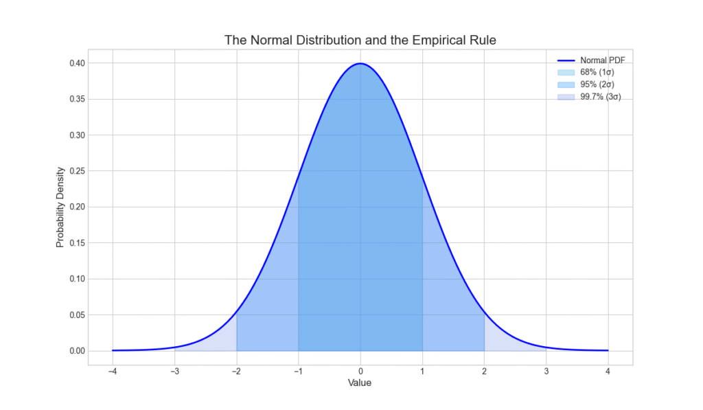
This visualization provides an intuitive grasp of how data is distributed around the mean in a Gaussian model, a concept vital for everything from statistical testing to setting anomaly detection thresholds.
Industry Applications and Case Studies
Probability theory is not just an academic exercise; it is actively deployed across industries to drive billions of dollars in value and solve critical problems.
- Financial Services: Risk Modeling and Algorithmic TradingIn finance, uncertainty is synonymous with risk. Banks and hedge funds use probability distributions to model the potential returns of assets. The Value at Risk (VaR) metric, for example, is often calculated using assumptions of normality (or more complex distributions like Student’s t-distribution to account for “fat tails”). It might state that “there is a 5% probability of the portfolio losing more than $1 million in one day.” Algorithmic trading systems use conditional probabilities and Bayesian models to predict short-term price movements based on a stream of market data, executing trades when the probability of a profitable outcome exceeds a certain threshold.
- Healthcare and Genomics: Diagnostic Systems and Gene SequencingAI-powered diagnostic tools use Bayes’ theorem to help physicians make better decisions. For a given patient with a set of symptoms (evidence), the system can calculate the posterior probability of various diseases (hypotheses). This requires knowledge of the prior probability of the disease in the population and the likelihood of observing those symptoms given the disease. In genomics, the Poisson distribution is used to model the occurrence of mutations or the number of DNA sequence reads aligning to a specific location in the genome, helping researchers identify significant genetic variations.
- Tech and E-commerce: Recommendation Engines and A/B TestingWhen Netflix recommends a movie, it’s not a deterministic choice. The system models the probability that you will enjoy and watch a particular title based on your viewing history and the behavior of similar users. This is a massive probabilistic inference problem. Similarly, companies like Amazon and Google use rigorous statistical hypothesis testing—grounded in probability theory—to conduct A/B tests. By showing different versions of a webpage to different users, they can determine with a certain level of confidence (e.g., 95%) whether a change like a new button color actually leads to a higher conversion rate (a Binomial success/failure outcome).
Best Practices and Common Pitfalls
While powerful, probabilistic methods must be applied with care and expertise. Misunderstanding or misusing these tools can lead to flawed conclusions and poorly performing AI systems.
- Choosing the Right Distribution: The “no free lunch” theorem applies here. No single distribution is perfect for all data. It is crucial to analyze your data’s characteristics. Is it count data (Poisson, Binomial)? Is it continuous and symmetric (Normal)? Is it skewed time-to-event data (Exponential, Weibull)? Visualizing your data with a histogram is a vital first step. Using a Normal distribution to model financial returns, for instance, is a common simplification that notoriously fails to capture the high frequency of extreme market events (fat tails).
- The Danger of the “Naive” Assumption: The conditional independence assumption in Naive Bayes is a powerful simplification, but it’s rarely true in the real world. In a spam filter, the words “free” and “money” are likely not independent. While the model often works well despite this, it’s important to be aware of the assumption’s limitations. When performance is critical and data is sufficient, more complex models like Bayesian Networks that can capture these dependencies should be considered.
- Correlation vs. Causation: This is a classic statistical pitfall. Just because two random variables move together (high correlation) does not mean one causes the other. A famous example is the high correlation between ice cream sales and drowning incidents. The confounding variable is temperature; hot weather causes both. Probabilistic models can reveal correlations, but establishing causality requires carefully designed experiments or more advanced causal inference methods.
- Interpreting p-values Correctly: In hypothesis testing, the p-value is the probability of observing data at least as extreme as what was collected, assuming the null hypothesis is true. It is not the probability that the null hypothesis is true. A small p-value (e.g., < 0.05) suggests that the observed data is unlikely under the null hypothesis, leading us to reject it. Misinterpreting p-values can lead to false discoveries and bad business decisions.
Tip: Always supplement statistical significance with effect size. A result can be statistically significant (low p-value) but have a tiny, practically meaningless effect size. For instance, an A/B test might show a new website design increases clicks with \(p=0.01\), but the actual increase might be only 0.001%, which is not worth the engineering cost to deploy.
Hands-on Exercises
These exercises are designed to reinforce the concepts in this chapter, progressing from theoretical calculation to practical implementation.
- Bayesian Inference by Hand: A rare disease affects 1 in 10,000 people. A test for this disease is 99% accurate (i.e., it correctly identifies a sick person 99% of the time and a healthy person 99% of the time). If a randomly selected person tests positive, what is the probability they actually have the disease?
- Objective: Apply Bayes’ theorem to a classic diagnostic problem.
- Hint: Define your events carefully: \(D\) = “has the disease”, \(+\) = “tests positive”. You need to find \(P(D|+)\). You are given \(P(D)\), \(P(+|D)\), and \(P(\text{no +}|\text{no D})\).
- Poisson Modeling of Website Traffic: A company’s website receives an average of 5 visitors per minute.
- Objective: Use the Poisson distribution to model real-world count data.
- Tasks:a. What is the probability of getting exactly 3 visitors in a given minute?b. What is the probability of getting 2 or fewer visitors in a given minute?c. Use scipy.stats.poisson to verify your calculations and plot the PMF for \(k\) from 0 to 15.
- Simulating the Central Limit Theorem:
- Objective: Gain an intuitive understanding of the Central Limit Theorem (CLT), one of the most profound results in probability.
- Tasks:a. Choose a non-normal distribution, for example, the Exponential distribution with \(\lambda=1\). Use numpy.random.exponential to draw 10,000 samples from it. Plot a histogram of these samples.b. Now, write a loop that runs 5,000 times. In each iteration, draw 30 samples from the same Exponential distribution and calculate their mean. Store these 5,000 means.c. Plot a histogram of the 5,000 sample means. What shape does it have? Compare it to the histogram from step (a).
- Expected Outcome: The histogram of individual samples will be highly skewed (characteristic of the Exponential distribution), but the histogram of the sample means will be bell-shaped, approximating a Normal distribution, thus demonstrating the CLT.
Tools and Technologies
A modern AI engineer’s toolkit for probability and statistics is primarily based in Python.
- NumPy: The fundamental package for numerical computing in Python. It provides efficient array objects and a vast library of mathematical functions. For probability,
numpy.randomis the workhorse for generating random numbers from various distributions and for simulating probabilistic systems. - SciPy: Built on top of NumPy,
scipy.statsis a comprehensive library for statistical functions and probability distributions. It provides tools for working with PMFs, PDFs, CDFs (Cumulative Distribution Functions), calculating moments, and performing statistical tests for dozens of common distributions. - Matplotlib & Seaborn: These are the primary plotting libraries in Python. Matplotlib provides fine-grained control over every aspect of a plot, while Seaborn offers a high-level interface for creating beautiful and informative statistical graphics, such as histograms, density plots, and regression plots.
- Statsmodels: A library that provides classes and functions for the estimation of many different statistical models, as well as for conducting statistical tests and statistical data exploration. It’s more focused on classical statistical modeling and econometrics than scikit-learn.
- PyMC & Stan (via cmdstanpy): For engineers focusing on Bayesian modeling, these are the state-of-the-art tools for Probabilistic Programming. They allow you to define complex Bayesian models in Python code and then use powerful inference algorithms (like Markov Chain Monte Carlo) to fit them to data.
Summary
This chapter established probability theory as a cornerstone of AI and machine learning, providing the tools to reason under uncertainty.
- Key Concepts: We formalized uncertainty using sample spaces, events, and the axioms of probability. We introduced conditional probability and the transformative Bayes’ theorem for updating beliefs.
- Random Variables: We defined discrete and continuous random variables and their key descriptors: PMF, PDF, expected value, and variance.
- Core Distributions: We explored the properties and applications of fundamental distributions in AI: Bernoulli, Binomial, Poisson for discrete data, and Uniform, Normal, Exponential for continuous data.
- Practical Skills: You learned to implement and visualize these concepts using Python’s scientific stack (NumPy, SciPy, Matplotlib), connecting abstract theory to concrete code.
- Real-World Relevance: We saw how probabilistic modeling drives value in finance, healthcare, and tech, and discussed the best practices and common pitfalls to ensure robust and reliable AI systems.
Further Reading and Resources
- Book: Probability Theory: The Logic of Science by E. T. Jaynes. A classic and profound treatment of probability as an extension of logic.
- Book: Introduction to Probability, 2nd Edition by Dimitri P. Bertsekas and John N. Tsitsiklis. A comprehensive and highly-rated undergraduate textbook used at MIT.
- Online Course: Stat 110: Probability by Joe Blitzstein (Harvard University). The complete course, including video lectures and notes, is available for free on YouTube and the course website.
- Documentation: The official documentation for
scipy.statsis an excellent and practical resource for exploring and using a wide range of probability distributions. https://docs.scipy.org/doc/scipy/reference/stats.html - Research Paper: “A Few Useful Things to Know About Machine Learning” by Pedro Domingos. Communications of the ACM, 2012. Provides high-level insights, including the importance of probabilistic thinking.
- Blog: Seeing Theory. An interactive online visualization of fundamental concepts in probability and statistics. (https://seeing-theory.brown.edu/)
- GitHub Repository: all-of-statistics. A collection of code implementations for the concepts in Larry Wasserman’s classic book “All of Statistics”.
Glossary of Terms
- Bayes’ Theorem: A mathematical formula for determining conditional probability. It describes how to update the probability of a hypothesis based on new evidence.
- Conditional Probability: The probability of an event occurring, given that another event has already occurred. Denoted \(P(A|B)\).
- Expected Value (E[X]): The long-run average value of a random variable; a measure of central tendency.
- Event: A subset of the sample space; a set of one or more possible outcomes of an experiment.
- Independence: The property of two events where the occurrence of one does not affect the probability of the other.
- Normal Distribution (Gaussian Distribution): A continuous probability distribution characterized by a symmetric, bell-shaped curve. It is defined by its mean \(\mu\) and standard deviation \(\sigma\).
- Probability Density Function (PDF): A function that describes the relative likelihood for a continuous random variable to take on a given value. The area under the curve between two points gives the probability for that range.
- Probability Mass Function (PMF): A function that gives the probability that a discrete random variable is exactly equal to some value.
- Random Variable: A variable whose value is a numerical outcome of a random phenomenon.
- Sample Space (\(\Omega\)): The set of all possible outcomes of a random experiment.
- Standard Deviation (\(\sigma\)): The square root of the variance; a measure of the amount of variation or dispersion of a set of values.
- Variance (\(\sigma^2\)): The expectation of the squared deviation of a random variable from its mean; a measure of spread.
