
Chapter 28: Outlier Detection and Treatment Methods
Chapter Objectives
Upon completing this chapter, you will be able to:
- Understand the theoretical foundations of outliers, including their various types, causes, and significant impact on statistical analysis and machine learning model performance.
- Implement a range of statistical and machine learning-based outlier detection techniques, including Z-score, Interquartile Range (IQR), Isolation Forest, and DBSCAN, using modern Python libraries.
- Analyze datasets to identify outliers, critically evaluating the suitability of different detection methods based on data characteristics and problem context.
- Design and apply appropriate treatment strategies for identified outliers, including removal, transformation, or imputation, justifying the choice based on analytical goals and business requirements.
- Optimize machine learning pipelines by integrating robust outlier detection and handling procedures, and evaluate their effect on model accuracy, stability, and generalizability.
- Deploy models with an awareness of how real-world data streams can introduce novel outliers, and incorporate strategies for monitoring and adapting to data drift.
Introduction
In the landscape of AI engineering, the quality of data is paramount. While we often focus on collecting vast quantities of information, the integrity of that data dictates the success or failure of any machine learning initiative. Among the most critical challenges in data preprocessing is the identification and management of outliers—data points that deviate so significantly from other observations as to arouse suspicion that they were generated by a different mechanism. These anomalies are not mere statistical curiosities; they are potent forces that can skew data distributions, bias parameter estimates, and ultimately degrade the predictive power of sophisticated algorithms. From a single fraudulent transaction that signals a security breach to a faulty sensor reading that could derail an autonomous vehicle, the ability to effectively manage outliers is a cornerstone of robust and reliable AI systems.
This chapter provides a comprehensive exploration of outlier detection and treatment, bridging statistical theory with practical, machine-learning-driven applications. We will move beyond simplistic definitions to understand the nuanced origins of outliers, recognizing that they can represent both data errors and critical, novel insights. We will delve into foundational statistical methods like the Z-score and Interquartile Range (IQR), which serve as a baseline for anomaly detection. Subsequently, we will advance to more sophisticated machine learning techniques, including the powerful Isolation Forest and density-based clustering with DBSCAN, which are designed to uncover complex, high-dimensional outliers that traditional methods may miss. By the end of this chapter, you will not only be equipped with a versatile toolkit for detecting anomalies but also with the critical judgment to decide their fate: whether to remove, transform, or embrace them as valuable signals in a noisy world. This knowledge is indispensable for building resilient, accurate, and trustworthy AI solutions that perform reliably in production environments.
Technical Background
Fundamental Concepts and Definitions
The journey into outlier analysis begins with a clear understanding of what constitutes an outlier and the profound effects these data points can have on our analytical models. An outlier is an observation that lies an abnormal distance from other values in a random sample from a population. This simple definition, however, belies a complex reality. The “abnormal distance” is subjective and highly dependent on the chosen detection method and the underlying data distribution. Outliers can manifest as univariate (an extreme value in a single feature) or multivariate (a surprising combination of values across multiple features). For instance, a person’s age of 150 is a univariate outlier, whereas an age of 15 combined with an annual income of $200,000 would be a multivariate outlier.
The origins of outliers are diverse. They can be genuine but extreme observations (e.g., the net worth of a billionaire in a sample of average citizens), which are part of the natural variation of the population. Alternatively, they can arise from measurement errors, data entry mistakes, or sampling errors. Distinguishing between these types is a critical, domain-specific task. An error should almost always be corrected or removed, while a genuine but extreme value may contain vital information. For example, in credit card fraud detection, the outlier—a transaction that deviates from a user’s normal spending pattern—is the very signal we aim to capture. Conversely, in a clinical trial, a data entry error in a patient’s blood pressure reading could lead to incorrect conclusions about a drug’s efficacy and must be handled carefully. The presence of outliers can severely impact statistical measures. The mean is notoriously sensitive to outliers, being pulled in the direction of the extreme value. The standard deviation and variance, which depend on the mean, are similarly affected, leading to an overestimation of variability. This distortion can invalidate the assumptions of many parametric statistical tests and machine learning algorithms, particularly linear models like linear regression and logistic regression, which assume normally distributed errors.

Core Terminology and Mathematical Foundations
To formalize our discussion, we must introduce key mathematical concepts. At the heart of many statistical detection methods is the assumption of a specific data distribution, most commonly the Gaussian (normal) distribution. A Gaussian distribution is defined by its mean, \(\mu\), and standard deviation, \(\sigma\). The probability density function is given by:
\[f(x \mid \mu, \sigma^2) = \frac{1}{\sqrt{2\pi\sigma^2}} e^{-\frac{(x-\mu)^2}{2\sigma^2}}\]
Under this assumption, we can quantify how “unlikely” a data point is. For example, in a standard normal distribution (where \(\mu=0\) and \(\sigma=1\)), approximately 68% of data falls within one standard deviation of the mean, 95% within two, and 99.7% within three. This is known as the empirical rule. A data point falling outside of \(\mu \pm 3\sigma\) is often considered a candidate for being an outlier.
The Z-score is a direct application of this principle. It measures how many standard deviations a data point \(x\) is from the mean \(\mu\). It is calculated as:
\[Z = \frac{x – \mu}{\sigma}\]
A common threshold for identifying an outlier is a Z-score with an absolute value greater than 3. However, this method has a critical weakness: the mean and standard deviation used in the calculation are themselves sensitive to the very outliers we are trying to detect. This phenomenon, known as masking, can cause the Z-score of a true outlier to be smaller than the threshold, thus hiding it.
To address this, robust statistics offer alternative measures that are less influenced by extreme values. The median is a robust measure of central tendency, and the Interquartile Range (IQR) is a robust measure of statistical dispersion. The IQR is the range between the first quartile (Q1, the 25th percentile) and the third quartile (Q3, the 75th percentile). An outlier is then often defined as any observation that falls outside the range:
\[[Q_1 – 1.5 \times IQR, Q_3 + 1.5 \times IQR]\]
The factor of 1.5 is a standard convention, but it can be adjusted. A more extreme range using a factor of 3.0 is sometimes used to identify “far out” or “extreme” outliers. Because the IQR method relies on percentiles, it is not distorted by a few extreme values, making it a more reliable choice for skewed or non-Gaussian data distributions.
Statistical and Proximity-Based Detection Methods
Building upon these foundational concepts, we can explore a broader class of detection methods. Statistical models, or parametric methods, assume an underlying distribution for the data. The goal is to find parameters for this distribution that best fit the majority of the data, and then identify points that have a low probability of being generated by this fitted model. The Z-score and IQR methods are simple examples of this approach. More advanced statistical methods might involve fitting a Gaussian Mixture Model (GMM), which represents the data as a combination of several Gaussian distributions. Points that do not fit well into any of the component distributions are flagged as outliers. The primary advantage of statistical methods is their mathematical rigor and efficiency, provided the assumptions about the data distribution hold true. Their main disadvantage is their inflexibility; if the true data distribution is different from the assumed one, the performance can be poor.
In contrast, proximity-based methods, which are non-parametric, make no prior assumptions about the data’s distribution. They operate on a simple, intuitive principle: outliers are data points that are isolated from the denser regions of the feature space. The effectiveness of these methods hinges on the choice of a distance metric, such as Euclidean distance or Manhattan distance, to quantify the proximity between points. A straightforward approach is to calculate the distance of each point to its k-th nearest neighbor (k-NN). Points with a large distance to their k-th nearest neighbor are considered outliers. This method is simple to understand and implement but suffers from the curse of dimensionality—in high-dimensional spaces, the concept of distance becomes less meaningful, and the computational cost of finding nearest neighbors becomes prohibitive, often scaling as \(O(n^2)\).
A more sophisticated and widely used proximity-based method is Density-Based Spatial Clustering of Applications with Noise (DBSCAN). DBSCAN groups together points that are closely packed, marking as outliers those points that lie alone in low-density regions. It defines points as core points, border points, or noise points (outliers) based on two parameters: eps (\(\epsilon\)), which specifies a radius, and min_samples, the minimum number of points required to form a dense region. A point is a core point if there are at least min_samples points within its \(\epsilon\)-neighborhood. A point is a border point if it is within the \(\epsilon\)-neighborhood of a core point but cannot form a dense region on its own. A noise point is any point that is neither a core nor a border point. DBSCAN is powerful because it can find arbitrarily shaped clusters and is robust to noise. Its primary challenge lies in selecting appropriate values for eps and min_samples, which can be non-intuitive and data-dependent.

Advanced Topics: Isolation Forest
While statistical and proximity-based methods are effective in many scenarios, they can struggle with high-dimensional data and large datasets. The Isolation Forest algorithm offers a fundamentally different and highly efficient approach specifically designed for anomaly detection. It operates on the principle that outliers are “few and different,” which makes them more susceptible to isolation than normal points. Instead of profiling normal data points, Isolation Forest explicitly tries to isolate anomalies.
The algorithm builds an ensemble of “Isolation Trees” (iTrees). To build an iTree, the algorithm recursively partitions the data by randomly selecting a feature and then randomly selecting a split value for that feature between the minimum and maximum values in the dataset. This random partitioning continues until a data point is isolated in a node by itself or a predefined tree height limit is reached. The intuition is that an outlier, being different, will require fewer random partitions to be isolated. A normal point, being embedded in a dense cluster of similar points, will require many more partitions to be singled out.
The anomaly score for a data point is derived from the average path length to isolate it across all the iTrees in the forest. The path length is the number of edges traversed from the root of the tree to a terminating node. The anomaly score \(s(x, n)\) for a point \(x\) is calculated as:
\[s(x,n) = 2 – \frac{E(h(x))}{c(n)}\]
where \(E(h(x))\) is the average path length of \(x\) over the ensemble of iTrees, and \(c(n)\) is the average path length of an unsuccessful search in a Binary Search Tree, used to normalize the score. The value of \(c(n)\) is given by:
\[c(n) = 2H(n-1) – \frac{2(n-1)}{n}\]
where \(H(i)\) is the harmonic number, which can be estimated as \(\ln(i) + 0.5772156649\) (Euler’s constant). The resulting anomaly score ranges between 0 and 1. A score close to 1 indicates a high likelihood of being an anomaly, a score much smaller than 0.5 suggests a normal point, and a score around 0.5 implies no strong distinction.
Isolation Forest has several key advantages. Its time complexity is linear, \(O(n)\), making it highly scalable. It does not rely on distance or density measures, which makes it effective in high-dimensional spaces. Furthermore, it requires very few parameters to tune—primarily the number of trees in the ensemble and the sub-sampling size. This makes it a powerful and easy-to-use first choice for many anomaly detection tasks.
flowchart TD
    A[Start with Dataset] --> B{Randomly Select Feature &<br>Randomly Select Split Value};

    B --> C{Partition Data};
    C --> D{Is Point Isolated?};

    subgraph "Path for Normal Point (Inlier)"
        D -- No --> E{...Many Partitions...};
        E --> F[Normal Point Isolated];
    end

    subgraph "Path for Anomalous Point (Outlier)"
       D -- Yes --> G[<b>Outlier Isolated</b>];
    end

    H["Calculate Anomaly Score<br><i>(Based on average path length across all trees)</i>"]
    F --> H;
    G --> H;
    H --> I{Score > Threshold?};
    I -- Yes --> J[Flag as Outlier];
    I -- No --> K[Flag as Inlier];

    classDef start fill:#283044,stroke:#283044,stroke-width:2px,color:#ebf5ee;
    classDef process fill:#78a1bb,stroke:#78a1bb,stroke-width:1px,color:#283044;
    classDef decision fill:#f39c12,stroke:#f39c12,stroke-width:1px,color:#283044;
    classDef endSuccess fill:#2d7a3d,stroke:#2d7a3d,stroke-width:2px,color:#ebf5ee;
    classDef endFail fill:#ebf5ee,stroke:#78a1bb,stroke-width:1px,color:#283044;
    classDef outlierPath fill:#e74c3c,stroke:#e74c3c,stroke-width:2px,color:#ebf5ee;

    class A start;
    class B,C,E,H process;
    class D,I decision;
    class J outlierPath;
    class G outlierPath;
    class K endFail;
    class F endFail;
Practical Examples and Implementation
This section translates the theoretical concepts of outlier detection into practical, executable code. We will use standard Python libraries such as NumPy for numerical operations, scikit-learn for machine learning models, and Matplotlib/Seaborn for visualization. These examples are designed to be run in a standard data science environment (e.g., a Jupyter Notebook).
Note: Ensure you have the necessary libraries installed. You can install them using pip:
Bashpip install numpy pandas scikit-learn matplotlib seaborn
Mathematical Concept Implementation
First, let’s implement the statistical methods—Z-score and the IQR rule—from scratch using NumPy to solidify our understanding of the underlying mathematics. We’ll generate some sample data with clear outliers.
import numpy as np
import pandas as pd

# Generate sample data: normal distribution with some outliers
np.random.seed(42)
data = np.random.randn(100) * 5 + 50  # Normal data centered around 50
# Add outliers
outliers = np.array([5, 10, 100, 105])
data_with_outliers = np.concatenate([data, outliers])

# --- Z-Score Implementation ---
def detect_outliers_zscore(data, threshold=3):
    """Detects outliers using the Z-score method."""
    mean = np.mean(data)
    std = np.std(data)
    outlier_indices = []
    for i, point in enumerate(data):
        z_score = (point - mean) / std
        if np.abs(z_score) > threshold:
            outlier_indices.append(i)
    return outlier_indices

zscore_outlier_indices = detect_outliers_zscore(data_with_outliers)
print(f"Outliers detected by Z-score (indices): {zscore_outlier_indices}")
print(f"Outlier values: {data_with_outliers[zscore_outlier_indices]}")

# --- IQR Implementation ---
def detect_outliers_iqr(data, factor=1.5):
    """Detects outliers using the IQR method."""
    q1 = np.percentile(data, 25)
    q3 = np.percentile(data, 75)
    iqr = q3 - q1
    lower_bound = q1 - (factor * iqr)
    upper_bound = q3 + (factor * iqr)

    outlier_indices = np.where((data < lower_bound) | (data > upper_bound))[0]
    return outlier_indices

iqr_outlier_indices = detect_outliers_iqr(data_with_outliers)
print(f"\nOutliers detected by IQR (indices): {iqr_outlier_indices}")
print(f"Outlier values: {data_with_outliers[iqr_outlier_indices]}")
Outputs:
Outliers detected by Z-score (indices): [100, 101, 102, 103]
Outlier values: [  5.  10. 100. 105.]

Outliers detected by IQR (indices): [ 74 100 101 102 103]
Outlier values: [ 36.90127448   5.          10.         100.         105.        ]
In this code, we first define functions to calculate outliers based on Z-score and IQR. The Z-score method correctly identifies the points 100 and 105 as outliers because their values are more than three standard deviations from the mean. The IQR method is more robust; it identifies all four injected points (5, 10, 100, 105) as outliers because they fall outside the \(1.5 \times IQR\) range from the quartiles. This demonstrates the IQR method’s superior ability to handle outliers without being unduly influenced by them.
Visualization and Interactive Examples
Visualization is a powerful tool for identifying and understanding outliers. A box plot is an excellent way to visualize the IQR method directly.
import numpy as np
import pandas as pd
import matplotlib.pyplot as plt
import seaborn as sns

# Generate sample data: normal distribution with some outliers
np.random.seed(42)
data = np.random.randn(100) * 5 + 50  # Normal data centered around 50
# Add outliers
outliers = np.array([5, 10, 100, 105])
data_with_outliers = np.concatenate([data, outliers])

# --- Z-Score Implementation ---
def detect_outliers_zscore(data, threshold=3):
    """Detects outliers using the Z-score method."""
    mean = np.mean(data)
    std = np.std(data)
    outlier_indices = []
    for i, point in enumerate(data):
        z_score = (point - mean) / std
        if np.abs(z_score) > threshold:
            outlier_indices.append(i)
    return outlier_indices

zscore_outlier_indices = detect_outliers_zscore(data_with_outliers)
print(f"Outliers detected by Z-score (indices): {zscore_outlier_indices}")
print(f"Outlier values: {data_with_outliers[zscore_outlier_indices]}")

# --- IQR Implementation ---
def detect_outliers_iqr(data, factor=1.5):
    """Detects outliers using the IQR method."""
    q1 = np.percentile(data, 25)
    q3 = np.percentile(data, 75)
    iqr = q3 - q1
    lower_bound = q1 - (factor * iqr)
    upper_bound = q3 + (factor * iqr)

    outlier_indices = np.where((data < lower_bound) | (data > upper_bound))[0]
    return outlier_indices

iqr_outlier_indices = detect_outliers_iqr(data_with_outliers)
print(f"\nOutliers detected by IQR (indices): {iqr_outlier_indices}")
print(f"Outlier values: {data_with_outliers[iqr_outlier_indices]}")


# Create a DataFrame for easier plotting
df = pd.DataFrame({'value': data_with_outliers})

plt.style.use('seaborn-v0_8-whitegrid')
fig, axes = plt.subplots(1, 2, figsize=(16, 6))

# Box plot
sns.boxplot(y='value', data=df, ax=axes[0])
axes[0].set_title('Box Plot of Data with Outliers')
axes[0].set_ylabel('Value')

# Scatter plot to show distribution
sns.scatterplot(x=range(len(df)), y='value', data=df, ax=axes[1], label='Data Points')
# Highlight outliers found by IQR
axes[1].scatter(iqr_outlier_indices, data_with_outliers[iqr_outlier_indices],
                color='red', s=100, label='IQR Outliers', zorder=5)
axes[1].set_title('Scatter Plot Highlighting IQR Outliers')
axes[1].set_xlabel('Index')
axes[1].set_ylabel('Value')
axes[1].legend()

plt.tight_layout()
plt.show()
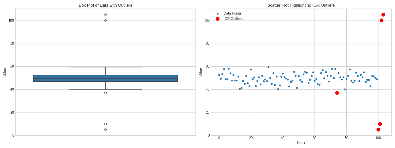
The box plot on the left clearly shows the four points as individual dots outside the “whiskers,” which represent the boundaries calculated using the IQR method. The scatter plot on the right provides another perspective, visually separating the red-highlighted outliers from the main cluster of data points.
AI/ML Application Examples
Now, let’s apply more advanced machine learning models from scikit-learn for outlier detection on a 2D dataset. We will use Isolation Forest and DBSCAN.
from sklearn.ensemble import IsolationForest
from sklearn.cluster import DBSCAN
from sklearn.preprocessing import StandardScaler

# Generate 2D sample data
np.random.seed(42)
X_normal = 0.3 * np.random.randn(100, 2)
# Create two clusters of normal data
X = np.r_[X_normal + 2, X_normal - 2]
# Add some random outliers
X_outliers = np.random.uniform(low=-4, high=4, size=(20, 2))
X_full = np.r_[X, X_outliers]

# --- Isolation Forest ---
# The 'contamination' parameter is the expected proportion of outliers
iso_forest = IsolationForest(n_estimators=100, contamination=0.1, random_state=42)
y_pred_iso = iso_forest.fit_predict(X_full)
# Predictions are -1 for outliers and 1 for inliers
iso_outliers = X_full[y_pred_iso == -1]

# --- DBSCAN ---
# Scale data for distance-based algorithms like DBSCAN
X_scaled = StandardScaler().fit_transform(X_full)
dbscan = DBSCAN(eps=0.4, min_samples=5)
y_pred_db = dbscan.fit_predict(X_scaled)
# Outliers are assigned the label -1
db_outliers = X_full[y_pred_db == -1]

# --- Visualization of ML Methods ---
fig, axes = plt.subplots(1, 2, figsize=(16, 7))

# Plot Isolation Forest results
axes[0].scatter(X_full[:, 0], X_full[:, 1], c='white', edgecolor='k', s=50)
axes[0].scatter(iso_outliers[:, 0], iso_outliers[:, 1], c='red', edgecolor='k', s=100, label='Outliers')
axes[0].set_title('Outlier Detection with Isolation Forest')
axes[0].legend()

# Plot DBSCAN results
axes[1].scatter(X_full[:, 0], X_full[:, 1], c='white', edgecolor='k', s=50)
axes[1].scatter(db_outliers[:, 0], db_outliers[:, 1], c='blue', edgecolor='k', s=100, label='Outliers')
axes[1].set_title('Outlier Detection with DBSCAN')
axes[1].legend()

plt.show()
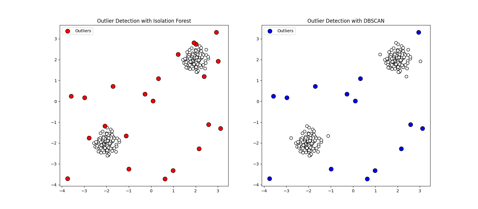
In this example, Isolation Forest successfully identifies most of the randomly scattered points as outliers (in red), as they are “different” and easily isolated. DBSCAN identifies outliers (in blue) as points that do not belong to any dense cluster. Note that some points near the main clusters are not flagged by DBSCAN, as its definition of an outlier is strictly tied to density. The choice between these methods depends on the problem: Isolation Forest is generally good for high-dimensional, global anomaly detection, while DBSCAN excels at finding noise points in clustered data.
Real-World Problem Applications and Treatment
Let’s consider a scenario of detecting anomalous sensor readings in an industrial IoT setting. Outliers could indicate a sensor malfunction or a critical event in the machinery. After detection, we must decide how to treat them.
flowchart TD
    A[Start: Outlier Detected] --> B{Is the outlier a result of<br>data entry or measurement error?};

    B -- Yes --> C{Can the correct value be determined?};
    C -- Yes --> D["Correct/Impute the value<br><i>(e.g., with mean, median, or model prediction)</i>"];
    C -- No --> E["Remove the data point<br><i>(Caution: only if dataset is large enough)</i>"];

    B -- No --> F{Is the outlier a genuine but extreme value?};
    F -- Yes --> G{Does the value skew the model<br>or violate its assumptions?};

    G -- Yes --> H["Transform the feature<br><i>(e.g., Log Transform, Winsorization)</i>"];
    G -- No --> I["Keep the data point<br><i>(It may contain valuable information)</i>"];

    F -- No --> J{"Is the outlier the primary signal of interest? <br><i>(e.g., Fraud, Intrusion)</i>"};
    J -- Yes --> K[Flag for investigation<br><b>Do not remove or alter</b>];
    J -- No --> L[Re-evaluate with domain expert];

    D --> M[End];
    E --> M[End];
    H --> M[End];
    I --> M[End];
    K --> M[End];
    L --> B;

    classDef start fill:#283044,stroke:#283044,stroke-width:2px,color:#ebf5ee;
    classDef decision fill:#f39c12,stroke:#f39c12,stroke-width:1px,color:#283044;
    classDef process fill:#78a1bb,stroke:#78a1bb,stroke-width:1px,color:#283044;
    classDef endSuccess fill:#2d7a3d,stroke:#2d7a3d,stroke-width:2px,color:#ebf5ee;
    classDef warning fill:#f1c40f,stroke:#f1c40f,stroke-width:1px,color:#283044;
    classDef model fill:#e74c3c,stroke:#e74c3c,stroke-width:1px,color:#ebf5ee;

    class A start;
    class B,C,F,G,J decision;
    class D,E,H,I,L process;
    class K model;
    class M endSuccess;
Treatment Strategies:
- Removal: If outliers are confirmed to be data entry errors or are corrupt, the simplest approach is to remove them. This is appropriate if the number of outliers is small, as removing too many points can lead to loss of information.
- Transformation: For genuine but extreme values that skew the data, transformations can be applied. A log transform (\(y = \log(x)\)) can pull in high values, while a square root transform can also stabilize variance. Another approach is winsorization, which caps the extreme values at a certain percentile (e.g., setting all values above the 99th percentile to the 99th percentile value).
- Imputation: If the outlier is an error but we cannot afford to lose the data point (e.g., in a time series), we can replace it with an imputed value, such as the mean, median, or a value predicted by a model.
- Keep them: In some cases, like fraud or intrusion detection, the outliers are the most important data points. In these scenarios, the goal is not to treat them but to flag them for further investigation.
Here is a code example demonstrating winsorization:
from scipy.stats.mstats import winsorize

# Use the 1D data from the first example
print(f"Original data (last 5 points): {data_with_outliers[-5:]}")

# Winsorize the data: cap values at the 5th and 95th percentiles
winsorized_data = winsorize(data_with_outliers, limits=[0.05, 0.05])

print(f"Winsorized data (last 5 points): {winsorized_data[-5:]}")

# Plotting the effect of Winsorization
fig, axes = plt.subplots(1, 2, figsize=(14, 5))
sns.histplot(data_with_outliers, kde=True, ax=axes[0], bins=20)
axes[0].set_title('Original Data Distribution')
sns.histplot(winsorized_data, kde=True, ax=axes[1], bins=20)
axes[1].set_title('Winsorized Data Distribution')
plt.show()
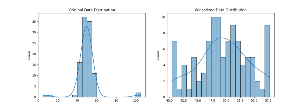
The output shows that the extreme values (like 105) have been replaced by the value at the 95th percentile of the original data. The histogram visualization confirms that the distribution is now less skewed, which can be beneficial for many machine learning models. The choice of treatment strategy is highly contextual and requires careful consideration of the data’s source and the project’s objectives.
Industry Applications and Case Studies
The principles of outlier detection are not merely academic; they are integral to the success of numerous high-stakes applications across various industries. Effective outlier management directly translates to reduced risk, enhanced security, and improved operational efficiency.
- Financial Services: Fraud Detection. In credit card and banking transactions, outliers are the primary signal of fraudulent activity. A transaction that is unusually large, occurs at an odd time, or originates from a new geographical location for a given user is a multivariate outlier. AI systems use models like Isolation Forest or autoencoders to score transactions in real-time. When a transaction’s anomaly score exceeds a threshold, it can be automatically blocked or flagged for manual review. The business impact is immense, saving financial institutions and consumers billions of dollars annually by preventing unauthorized transactions. The technical challenge lies in minimizing false positives (legitimate transactions incorrectly flagged as fraud) to avoid inconveniencing customers.
- Cybersecurity: Network Intrusion Detection. Network traffic data is monitored for patterns that deviate from the norm. An outlier could be a sudden spike in data packets from a single IP address, an attempt to access an unusual port, or a data transfer of an abnormally large size. These anomalies can indicate a denial-of-service (DoS) attack, a malware infection, or data exfiltration. Proximity-based and density-based methods like DBSCAN are effective here for identifying anomalous clusters of network activity. The ROI is measured in the prevention of data breaches, which can cost companies millions in damages, regulatory fines, and reputational harm.
- Manufacturing: Predictive Maintenance. In industrial IoT, sensors on machinery continuously stream data like temperature, vibration, and pressure. An outlier in this time-series data can be an early indicator of an impending equipment failure. For example, a sudden, sharp increase in vibration might signal a bearing is about to fail. Statistical methods and time-series anomaly detection algorithms are used to monitor these streams. By detecting these outliers, companies can perform maintenance proactively, avoiding costly unplanned downtime and extending the lifespan of their equipment.
- Healthcare: Medical Diagnosis. In medical imaging, an outlier could be a region in an MRI or CT scan that has different textural properties, potentially indicating a tumor. In patient electronic health records, an anomalous combination of lab results and vital signs could signal the onset of a serious condition like sepsis. Machine learning models are trained on vast amounts of patient data to learn what constitutes a “normal” physiological state, allowing them to flag high-risk patients for immediate attention from medical professionals, thereby improving patient outcomes.
Best Practices and Common Pitfalls
Developing a robust outlier detection and treatment strategy requires more than just applying an algorithm; it demands careful thought, domain expertise, and adherence to best practices. Mismanaging outliers can be as detrimental as ignoring them.
- Context is King: Involve Domain Experts. An outlier is only meaningful in context. A value that is anomalous in one domain may be perfectly normal in another. Always consult with domain experts to understand the data-generating process. They can help distinguish between data errors, measurement noise, and genuinely novel events. This collaboration is crucial for deciding whether an outlier should be removed, corrected, or investigated further.
- Visualize, Visualize, Visualize. Before applying any automated detection algorithm, visually inspect your data. Simple plots like histograms, box plots, and scatter plots can often reveal obvious outliers and provide intuition about the data’s distribution. For high-dimensional data, use dimensionality reduction techniques like PCA or t-SNE to create 2D or 3D visualizations. This initial exploratory step can prevent you from choosing an inappropriate method.
- Avoid One-Size-Fits-All Thresholds. The thresholds used in methods like Z-score (e.g.,
|Z| > 3) or IQR (e.g., the 1.5 factor) are rules of thumb, not immutable laws. The optimal threshold depends on the specific dataset and the tolerance for false positives versus false negatives. It’s often better to treat anomaly scores as a ranking and investigate the top N most anomalous points, rather than relying on a rigid cutoff. - Consider the Impact on Your Model. The choice of outlier treatment should be guided by the machine learning model you intend to use. Tree-based models like Random Forests and Gradient Boosting are generally robust to outliers and may not require explicit handling. In contrast, linear models and distance-based algorithms like K-Means or SVM are highly sensitive to them. Always evaluate your model’s performance with and without outlier treatment to make an informed decision.
- Don’t Test on Your Training Set’s Outliers. When splitting your data, perform outlier detection and removal after the split, and apply it only to the training set. Outliers in the test or validation set represent the kind of unexpected data your model might encounter in the real world. Removing them from the test set will give you an overly optimistic estimate of your model’s performance. The treatment strategy (e.g., transformation parameters) learned from the training data should then be applied to the test data.
- Document Everything. Keep a meticulous record of the outlier detection methods you used, the parameters and thresholds chosen, and the treatment strategies applied. This documentation is vital for reproducibility, for explaining your modeling decisions to stakeholders, and for debugging when the model behaves unexpectedly in production.
Hands-on Exercises
- Beginner: Financial Transaction Analysis.
- Objective: Identify potentially fraudulent transactions using basic statistical methods.
- Dataset: You are given a CSV file
transactions.csvwith columnstransaction_id,user_id, andamount. - Task:
- Load the data into a pandas DataFrame.
- Calculate the Z-score for the
amountcolumn. - Identify all transactions with a Z-score greater than 3.5.
- Use the IQR method with a factor of 2.0 to identify outliers.
- Print the transaction IDs identified by both methods. Are they the same? Why might they differ?
- Verification: Your output should be two lists of transaction IDs. You should be able to explain why the stricter Z-score threshold might find fewer outliers than the IQR method.
- Intermediate: Multi-dimensional Sensor Data.
- Objective: Apply machine learning-based outlier detection on a multi-dimensional dataset.
- Dataset: A dataset
sensor_data.csvcontains readings from three sensors:temp,vibration, andpressure. - Task:
- Load and visualize the data using a 3D scatter plot.
- Standardize the data using
StandardScaler. - Apply the Isolation Forest algorithm. Experiment with the
contaminationparameter (e.g., 0.05, 0.1). - Apply the DBSCAN algorithm. You will need to experiment with the
epsandmin_samplesparameters to get meaningful results. A good starting point might be to use a k-NN plot to estimateeps. - Create scatter plots highlighting the outliers detected by each method. Discuss the differences in the points they identified.
- Verification: You should produce visualizations showing the outliers flagged by both models and provide a written analysis comparing their results.
- Advanced (Team Project): Building a Robust Preprocessing Pipeline.
- Objective: Design and implement a reusable Python class for outlier detection and treatment.
- Task:
- Design a
DataCleanerclass in Python. - The class constructor (
__init__) should take a pandas DataFrame as input. - Implement methods within the class for different detection techniques (e.g.,
detect_outliers_iqr(),detect_outliers_isoforest()). These methods should return the indices of the detected outliers. - Implement treatment methods like
remove_outliers(indices)andtransform_winsorize(column, limits). - The class should maintain a log of all operations performed (e.g., “Removed 15 outliers from ‘amount’ using IQR method.”).
- Apply your
DataCleanerclass to a real-world dataset (e.g., from Kaggle). Demonstrate a full workflow: load data, detect outliers using multiple methods, apply a treatment, and show the data distribution before and after.
- Design a
- Verification: The final deliverable is a well-documented Python script containing the
DataCleanerclass and a Jupyter Notebook demonstrating its application and effectiveness on a chosen dataset.
Tools and Technologies
The primary tool for outlier detection in Python is the rich ecosystem of data science libraries.
- scikit-learn: This is the cornerstone library for machine learning in Python. It provides robust, well-documented implementations of several key outlier detection algorithms.
sklearn.ensemble.IsolationForest: The go-to implementation for Isolation Forest.sklearn.cluster.DBSCAN: For density-based outlier detection.sklearn.neighbors.LocalOutlierFactor: Another powerful proximity-based method that computes a score reflecting the local density deviation of a data point with respect to its neighbors.sklearn.preprocessing.StandardScaler: Essential for preprocessing data before applying distance-based algorithms.
- PyOD (Python Outlier Detection): For more advanced or specialized needs, PyOD is a comprehensive and dedicated toolkit for outlier detection. It provides access to over 30 different algorithms, from classical methods to the latest deep learning-based approaches. It integrates seamlessly with the scikit-learn API.Tip: If your project requires comparing multiple outlier detection algorithms or using more niche techniques, PyOD is an excellent choice. Installation is simple:
pip install pyod. - NumPy & pandas: These libraries are fundamental for data manipulation, cleaning, and performing the mathematical calculations required for statistical methods.
- Matplotlib & Seaborn: These are the standard libraries for data visualization in Python. They are indispensable for the exploratory analysis step and for communicating the results of your outlier detection process.
- SciPy: This library is useful for more advanced statistical functions, including
scipy.stats.mstats.winsorizefor data transformation and various statistical tests that can help in understanding your data’s distribution.
A typical development workflow involves using pandas to load and clean data, Matplotlib/Seaborn to visualize it, and then applying a detection algorithm from scikit-learn or PyOD. The choice of tool depends on the complexity of the task and the specific characteristics of the dataset.
Summary
- Outliers are data points that deviate significantly from the rest of the data. They can be errors or genuine, novel events, and their presence can severely distort statistical analyses and machine learning models.
- Detection methods range from simple statistical rules to complex machine learning algorithms. Statistical methods like Z-score and IQR are fast and interpretable but rely on assumptions about the data’s distribution.
- Machine learning approaches offer more power and flexibility. Isolation Forest is highly efficient and effective for high-dimensional data by isolating anomalies. DBSCAN identifies outliers as noise points in low-density regions.
- Outlier treatment is context-dependent. Strategies include removal (for errors), transformation (like winsorization or log transforms to reduce skew), imputation, or keeping them as the primary signal of interest (e.g., in fraud detection).
- Best practices are crucial for robust outlier management. This includes involving domain experts, visualizing data, avoiding rigid thresholds, and carefully considering the impact on the specific ML model being used.
- Practical implementation relies on a standard Python data science stack, including scikit-learn, NumPy, pandas, and visualization libraries, with PyOD available for more advanced use cases.
Comparison of Outlier Detection Methods
| Method | Underlying Principle | Data Assumptions | Strengths | Weaknesses |
|---|---|---|---|---|
| Z-Score | Statistical (Parametric) | Assumes a Gaussian (normal) distribution. | – Simple and fast to compute. – Easy to interpret. |
– Highly sensitive to outliers (masking effect). – Not suitable for non-Gaussian data. |
| IQR | Statistical (Non-Parametric) | No specific distribution assumed. | – Robust to outliers. – Works well for skewed distributions. |
– Only for univariate analysis. – Can be too aggressive/conservative based on the 1.5 factor. |
| DBSCAN | Density-Based | No distribution assumed. Identifies low-density regions. | – Can find arbitrarily shaped clusters. – Does not require specifying the number of clusters. |
– Performance depends heavily on eps and min_samples parameters. – Struggles with varying density clusters. |
| Isolation Forest | Partitioning-Based (Ensemble) | No distribution assumed. Based on ease of isolation. | – Highly efficient and scalable (linear time complexity). – Effective in high-dimensional spaces. – Requires few parameters. |
– May struggle with complex datasets where outliers and inliers are not easily separable. |
Further Reading and Resources
- Aggarwal, Charu C. Outlier Analysis. Springer, 2017. The most comprehensive academic textbook on the topic, covering a vast range of algorithms and theories.
- Scikit-learn User Guide: Novelty and Outlier Detection. The official documentation provides excellent explanations and examples for the outlier detection algorithms implemented in the library. (https://scikit-learn.org/stable/modules/outlier_detection.html)
- PyOD GitHub Repository and Documentation. An essential resource for exploring a wider variety of outlier detection algorithms and their implementations. (https://github.com/yzhao062/pyod)
- “How to Use and Create a Box Plot” by Towards Data Science. A practical, well-explained tutorial on using box plots for outlier visualization. (A search for this title on the platform will yield numerous high-quality articles).
- Chandola, Varun, Arindam Banerjee, and Vipin Kumar. “Anomaly detection: A survey.” ACM computing surveys (CSUR) 41.3 (2009): 1-58. A highly cited survey paper that provides a structured overview of the field.
- Liu, Fei Tony, Kai Ming Ting, and Zhi-Hua Zhou. “Isolation forest.” 2008 Eighth IEEE International Conference on Data Mining. IEEE, 2008. The original research paper that introduced the Isolation Forest algorithm.
Glossary of Terms
- Anomaly: A synonym for an outlier; a data point that deviates from a well-defined notion of normal behavior.
- DBSCAN (Density-Based Spatial Clustering of Applications with Noise): A clustering algorithm that groups together points that are closely packed, marking as outliers points that lie alone in low-density regions.
- Inlier: A data point that is not an outlier and belongs to the normal distribution of the data.
- Interquartile Range (IQR): A measure of statistical dispersion, being equal to the difference between the 75th (Q3) and 25th (Q1) percentiles.
- Isolation Forest: A machine learning algorithm for anomaly detection that works by randomly partitioning the data to isolate outliers.
- Masking Effect: A phenomenon where the presence of one or more outliers inflates the statistical measures (like mean and standard deviation) used for detection, causing other outliers to be missed.
- Multivariate Outlier: An outlier that is identified by an unusual combination of values across multiple features or variables.
- Robust Statistics: Statistical methods that are resistant to the influence of outliers. The median and IQR are examples of robust statistics.
- Univariate Outlier: An outlier that is an extreme value for a single feature or variable.
- Winsorization: The process of transforming data by limiting extreme values to reduce the effect of outliers. It involves setting all outliers to a specified percentile of the data.
- Z-score: A statistical measurement that describes a value’s relationship to the mean of a group of values, measured in terms of standard deviations from the mean.
