
Chapter 17: Convex Optimization and Lagrange Multipliers
Chapter Objectives
Upon completing this chapter, students will be able to:
- Understand the fundamental principles of convex optimization, including convex sets, convex functions, and the properties that make these problems computationally tractable.
- Analyze constrained optimization problems by formulating the Lagrangian function and applying the Karush-Kuhn-Tucker (KKT) conditions to find optimal solutions.
- Implement solutions to convex optimization problems in Python using standard scientific computing libraries such as NumPy, SciPy, and CVXPY.
- Design and interpret machine learning models, such as Support Vector Machines (SVMs), by understanding their underlying constrained optimization formulation.
- Evaluate the role of duality in optimization, explain the relationship between primal and dual problems, and leverage it to solve complex problems more efficiently.
- Apply optimization principles to real-world AI engineering problems, including regularization techniques in linear models and resource allocation challenges.
Introduction
Optimization is the heart of modern machine learning. At its core, “learning” from data is an optimization problem: we seek a set of model parameters that minimizes a loss function, thereby maximizing the model’s performance on a given task. While methods like gradient descent provide a powerful tool for unconstrained optimization, many of the most influential algorithms in AI are defined by constraints. How do we find the best solution when our choices are limited to a specific region or must satisfy certain conditions? This is the central question of constrained optimization, a field that provides the theoretical and practical machinery for solving some of the most important problems in AI engineering.
This chapter delves into convex optimization, a special class of optimization problems that is both mathematically elegant and computationally efficient. Unlike general non-convex problems, which can be riddled with local minima that trap algorithms, convex problems guarantee that any local minimum is also a global minimum. This remarkable property is the reason why so many machine learning models, from Support Vector Machines to logistic regression, are formulated as convex problems. We will explore the foundational concepts of convex sets and functions before introducing the powerful method of Lagrange multipliers and the more general Karush-Kuhn-Tucker (KKT) conditions. These tools allow us to systematically solve problems with equality and inequality constraints. By understanding this mathematical framework, you will gain a profound insight into not just how algorithms like SVMs work, but why they are designed the way they are, unlocking the ability to analyze, customize, and innovate in the field of AI.
        graph TD
            A[Start: Define Real-World Problem] --> B{Formulate Mathematically};
            B --> C["Identify: <br>1. Objective Function f(x)<br>2. Equality Constraints h(x)<br>3. Inequality Constraints g(x)"];
            C --> D{Is the problem convex?};
            D -- Yes --> E["Construct the Lagrangian<br>L(x, μ, λ)"];
            E --> F[Apply KKT Conditions<br>1. Stationarity<br>2. Primal Feasibility<br>3. Dual Feasibility<br>4. Complementary Slackness];
            F --> G[Solve the resulting<br>system of equations];
            G --> H((Optimal Solution x*));
            D -- No --> I["Use general non-linear solvers<br><i>(e.g., SLSQP)</i>"];
            I --> J((Local Optimum Found));
            H --> K[End: Interpret Solution];
            J --> K;

            %% Styling
            classDef primary fill:#283044,stroke:#283044,stroke-width:2px,color:#ebf5ee;
            classDef success fill:#2d7a3d,stroke:#2d7a3d,stroke-width:2px,color:#ebf5ee;
            classDef decision fill:#f39c12,stroke:#f39c12,stroke-width:1px,color:#283044;
            classDef process fill:#78a1bb,stroke:#78a1bb,stroke-width:1px,color:#283044;
            classDef warning fill:#f1c40f,stroke:#f1c40f,stroke-width:1px,color:#283044;

            class A,K primary;
            class H,J success;
            class D decision;
            class I warning;
            class B,C,E,F,G process;
Technical Background
Fundamental Concepts of Optimization
At its most abstract level, an optimization problem involves finding the best solution from a set of all feasible solutions. This is formalized by defining an objective function, which we aim to minimize or maximize, and a set of constraints that define the space of valid solutions. The journey into the mechanics of machine learning is, in essence, a journey through the landscape of optimization. The models we build are defined by parameters, and the process of training is the search for the optimal parameter values that minimize a loss function—a measure of the model’s error.
Core Terminology and Mathematical Foundations
A general optimization problem can be expressed as:
\[\begin{aligned} & \underset{x}{\text{minimize}} & & f_0(x) \\ & \text{subject to} & & f_i(x) \leq 0, \quad i = 1, \ldots, m \\ & & & h_j(x) = 0, \quad j = 1, \ldots, p \end{aligned}\]
Here, \(x \in \mathbb{R}^n\) is the optimization variable, a vector of parameters we are adjusting. The function \(f_0(x): \mathbb{R}^n \to \mathbb{R}\) is the objective function that we want to minimize. The functions \(f_i(x) \leq 0\) are the inequality constraints, and \(h_j(x) = 0\) are the equality constraints. The set of all points \(x\) that satisfy all constraints is called the feasible set.
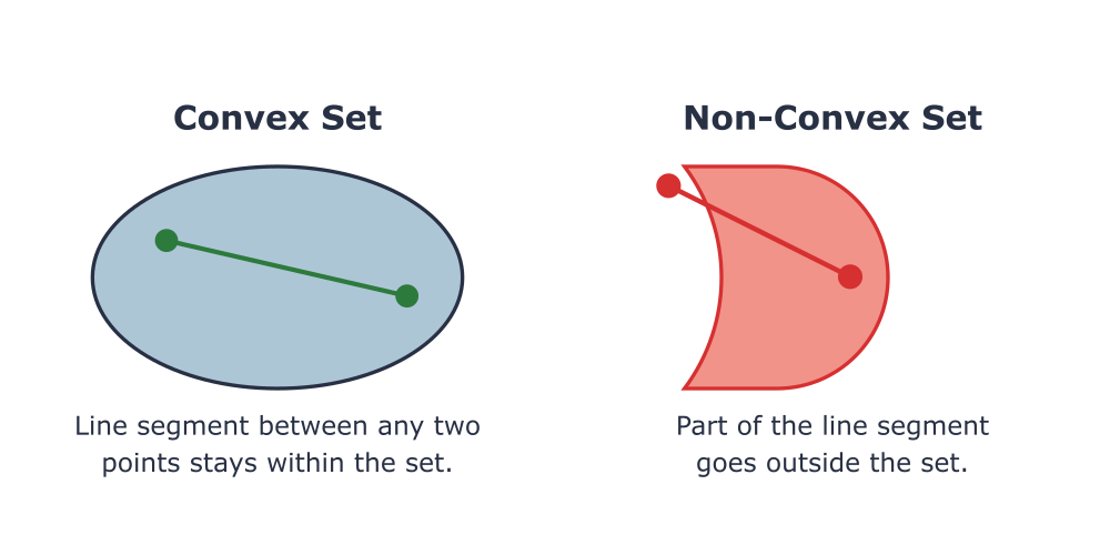
The true power in optimization for machine learning comes when we can provide guarantees about the solutions we find. This is where the concept of convexity becomes paramount. A convex set \(C\) is a set of points where for any two points \(x, y \in C\), the line segment connecting them, \(\theta x + (1-\theta)y\) for \(0 \leq \theta \leq 1\), is also entirely contained within \(C\). Geometrically, a convex set has no “dents” or “holes.” A convex function is one where the region above its graph is a convex set. Formally, a function \(f\) is convex if for any \(x, y\) in its domain and for \(0 \leq \theta \leq 1\), the following inequality holds:
\[ f(\theta x + (1-\theta)y) \leq \theta f(x) + (1-\theta)f(y) \]
This inequality states that the function’s value at any point on the line segment between \(x\) and \(y\) is less than or equal to the value of the line segment connecting \(f(x)\) and \(f(y)\). For a differentiable function, this is equivalent to its Hessian matrix (the matrix of second partial derivatives) being positive semidefinite.
A convex optimization problem is one where the objective function is convex, the inequality constraint functions are convex, and the equality constraint functions are affine (i.e., linear, of the form \(Ax – b = 0\)). The crucial property of these problems is that any locally optimal solution is also a globally optimal solution. This eliminates the pervasive issue of getting stuck in suboptimal solutions, which plagues non-convex optimization (such as in the training of deep neural networks).
Historical Development and Evolution
The roots of optimization are ancient, but its modern formulation began in the 18th century with the work of mathematicians like Leonhard Euler and Joseph-Louis Lagrange. Lagrange, in particular, developed a method for handling equality constraints in calculus of variations, which laid the groundwork for the method of Lagrange multipliers. His insight was that at a constrained optimum, the gradient of the objective function must be a linear combination of the gradients of the constraint functions. This geometric intuition remains the cornerstone of constrained optimization theory.
The field took a significant leap forward in the mid-20th century. The development of the simplex algorithm for Linear Programming (LP) by George Dantzig in the 1940s revolutionized industries by enabling the optimization of complex logistics and resource allocation problems. The theory was further generalized in the 1950s by Harold W. Kuhn and Albert W. Tucker, who, building on the earlier work of William Karush, developed the Karush-Kuhn-Tucker (KKT) conditions. These conditions extend Lagrange’s method to handle both equality and inequality constraints, forming the bedrock of modern non-linear programming. The advent of powerful computers and the development of interior-point methods in the 1980s made it possible to solve large-scale convex optimization problems efficiently, paving the way for their widespread adoption in machine learning, finance, and engineering.
Constrained Optimization and Duality
While unconstrained optimization methods like gradient descent are foundational, they cannot handle problems where the solution must adhere to specific rules. Constrained optimization provides the framework for this, and the concept of duality offers a powerful alternative perspective for solving these problems.
Equality Constraints and the Lagrangian
Consider a simple problem with only equality constraints: minimize \(f(x)\) subject to \(h(x) = 0\). At an optimal point \(x^*\), we cannot move in any direction that is tangent to the constraint surface \(h(x) = 0\) and decrease \(f(x)\). This implies that at \(x^*\), the gradient of the objective function, \(\nabla f(x^*)\), must be orthogonal to the constraint surface. The gradient of the constraint function, \(\nabla h(x^*)\), is also orthogonal to the constraint surface. Therefore, the two gradients must be parallel, meaning one is a scalar multiple of the other:
\[ \nabla f(x^*) + \lambda \nabla h(x^*) = 0 \]
The scalar \(\lambda\) is called the Lagrange multiplier. This geometric condition is elegantly captured by constructing a new function, the Lagrangian:
\[ \mathcal{L}(x, \lambda) = f(x) + \lambda h(x) \]
We can then find the optimal point by solving the unconstrained problem of finding the stationary points of the Lagrangian, i.e., where its gradient with respect to both \(x\) and \(\lambda\) is zero:
\[ \nabla_x \mathcal{L}(x, \lambda) = \nabla f(x) + \lambda \nabla h(x) = 0 \]
\[ \nabla_\lambda \mathcal{L}(x, \lambda) = h(x) = 0 \]
Solving this system of equations gives us the candidate optimal points. The Lagrange multiplier \(\lambda\) can be interpreted as the rate of change of the optimal objective value with respect to a change in the constraint, often called a “shadow price.”

Inequality Constraints and the KKT Conditions
When we introduce inequality constraints, \(g(x) \leq 0\), the situation becomes more complex. An inequality constraint can be either active (i.e., \(g(x) = 0\) at the optimum) or inactive (i.e., \(g(x) < 0\) at the optimum).
- If a constraint is inactive, the optimal point lies in the interior of the feasible region for that constraint, so the constraint has no influence. It is as if it wasn’t there, and its corresponding Lagrange multiplier is zero.
- If a constraint is active, the optimum lies on the boundary defined by that constraint. The situation is similar to an equality constraint, and the gradient of the objective must point “away” from the feasible region.
The Karush-Kuhn-Tucker (KKT) conditions provide a comprehensive set of necessary conditions for optimality in problems with both equality and inequality constraints. For the general problem stated earlier, the Lagrangian is:
\[ \mathcal{L}(x, \mu, \lambda) = f_0(x) + \sum_{i=1}^{m} \mu_i f_i(x) + \sum_{j=1}^{p} \lambda_j h_j(x) \]
The KKT conditions for an optimal point \(x^*\) are:
- Stationarity: The gradient of the Lagrangian with respect to \(x\) is zero: \(\nabla_x \mathcal{L}(x^, \mu^, \lambda^*) = 0\).
- Primal Feasibility: The original constraints must be satisfied: \(f_i(x^) \leq 0\) and \(h_j(x^) = 0\).
- Dual Feasibility: The Lagrange multipliers for the inequality constraints must be non-negative: \(\mu_i^* \geq 0\). This ensures the objective gradient points away from the feasible region for active constraints.
- Complementary Slackness: For each inequality constraint, either the constraint is active or its multiplier is zero: \(\mu_i^* f_i(x^*) = 0\). This elegantly combines the active and inactive cases.
For convex problems, the KKT conditions are not just necessary but also sufficient for optimality. This makes them an incredibly powerful tool for both analyzing and solving machine learning problems.
Duality in Optimization
Duality provides a different lens through which to view a constrained optimization problem. Every optimization problem, referred to as the primal problem, has an associated dual problem. The dual problem is formulated by defining the Lagrange dual function, \(g(\mu, \lambda)\), which is the minimum value of the Lagrangian over \(x\):
\[ g(\mu, \lambda) = \inf_{x} \mathcal{L}(x, \mu, \lambda) \]
The dual problem is then to maximize this dual function, subject to the dual feasibility constraints:
\[\begin{aligned} & \underset{\mu, \lambda}{\text{maximize}} & & g(\mu, \lambda) \\ & \text{subject to} & & \mu_i \geq 0, \quad i = 1, \ldots, m \end{aligned}\]
A key property is that the dual function is always concave, regardless of whether the primal problem is convex. This means the dual problem is a convex optimization problem, which can be easier to solve. The optimal value of the dual problem, \(d^*\), provides a lower bound on the optimal value of the primal problem, \(p^*\). This is known as weak duality: \(d^* \leq p^*\).
For most convex optimization problems that satisfy certain regularity conditions (like Slater’s condition, which states there exists a strictly feasible point), strong duality holds: \(d^* = p^*\). When strong duality holds, we can solve the dual problem to find the optimal value of the primal. This is not just a theoretical curiosity; it has profound practical implications. As we will see with Support Vector Machines, solving the dual problem can be much more efficient and can reveal deep structural insights about the solution, leading to powerful concepts like the kernel trick.
Practical Examples and Implementation
Theory becomes tangible when implemented in code. This section translates the mathematical concepts of convex optimization and Lagrange multipliers into practical Python implementations using standard libraries. We will see how these foundational ideas power real machine learning algorithms.
Mathematical Concept Implementation
We can use Python libraries to solve constrained optimization problems directly. SciPy provides a robust optimize module, and for problems that can be explicitly formulated as convex, CVXPY offers a more powerful and expressive domain-specific language.
Let’s solve a simple quadratic programming problem:
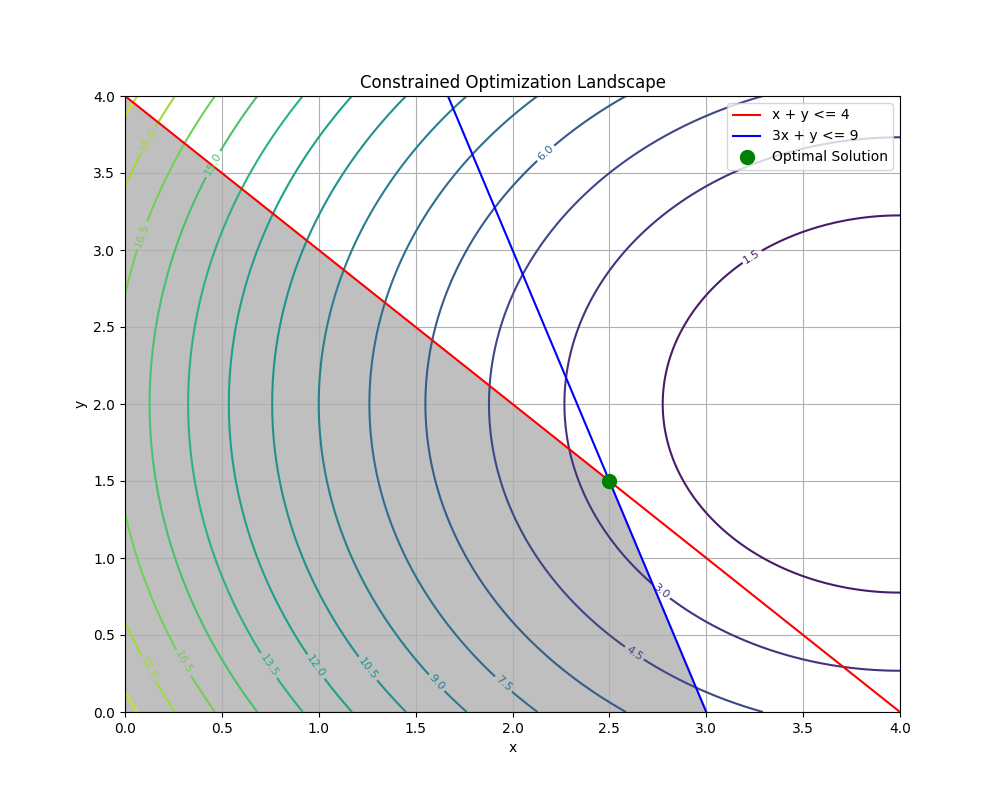
Minimize \(f(x, y) = (x-4)^2 + (y-2)^2\) subject to the constraints:
- \(x + y \leq 4\)
- \(3x + y \leq 9\)
- \(x \geq 0, y \geq 0\)
This is a convex optimization problem because the objective function is a convex quadratic, and the constraints are linear (and therefore affine).
import numpy as np
from scipy.optimize import minimize

# Define the objective function
def objective(x):
    return (x[0] - 4)**2 + (x[1] - 2)**2

# Define the constraints
# Note: scipy.optimize.minimize expects constraints in the form g(x) >= 0
# So we rewrite x + y <= 4 as 4 - x - y >= 0
# and 3x + y <= 9 as 9 - 3x - y >= 0
cons = ({'type': 'ineq', 'fun': lambda x: 4 - x[0] - x[1]},
        {'type': 'ineq', 'fun': lambda x: 9 - x[0]*3 - x[1]})

# Define the bounds for the variables (x >= 0, y >= 0)
bnds = ((0, None), (0, None))

# Initial guess
x0 = np.array([0.5, 0.5])

# Solve the optimization problem
solution = minimize(objective, x0, method='SLSQP', bounds=bnds, constraints=cons)

# Print the results
if solution.success:
    print("Optimal solution found:")
    print(f"x = {solution.x[0]:.4f}, y = {solution.x[1]:.4f}")
    print(f"Objective value = {solution.fun:.4f}")
else:
    print("Optimization failed:", solution.message)

# Let's check which constraints are active at the solution
x_opt = solution.x
print("\nChecking constraints at the optimal point:")
print(f"Constraint 1 (x + y <= 4): {x_opt[0] + x_opt[1]:.4f}")
print(f"Constraint 2 (3x + y <= 9): {x_opt[0]*3 + x_opt[1]:.4f}")
Output:
ptimal solution found:
x = 2.5000, y = 1.5000
Objective value = 2.5000

Checking constraints at the optimal point:
Constraint 1 (x + y <= 4): 4.0000
Constraint 2 (3x + y <= 9): 9.0000
Note: The
SLSQP(Sequential Least Squares Programming) method is a powerful algorithm suitable for general non-linear constrained optimization. It can handle both convex and non-convex problems, but for convex problems, it reliably finds the global optimum.
AI/ML Application Examples
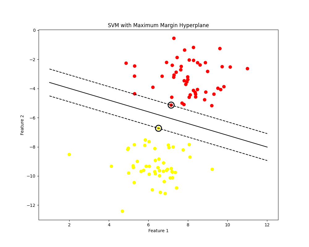
The most classic application of constrained optimization and duality in machine learning is the Support Vector Machine (SVM). The goal of a linear SVM is to find a hyperplane that separates two classes of data with the maximum possible margin.
The margin is the distance between the hyperplane and the closest data points from either class. Maximizing the margin leads to better generalization. Let the hyperplane be defined by \(w^T x – b = 0\). We want to maximize the margin, which is equivalent to minimizing \(\frac{1}{2} ||w||^2\), subject to the constraint that all data points are correctly classified and are at least a distance of 1 (in a scaled sense) from the hyperplane. For data points \((x_i, y_i)\) where \(y_i \in {-1, 1}\), this constraint is \(y_i(w^T x_i – b) \geq 1\).
This is a convex quadratic programming problem. By forming the Lagrangian and solving the dual problem, we discover something remarkable: the solution for \(w\) is a linear combination of only a few of the input data points, those that lie exactly on the margin boundary. These are the support vectors. This is a direct consequence of the complementary slackness condition from KKT.
import numpy as np
import matplotlib.pyplot as plt
from sklearn.svm import SVC
from sklearn.datasets import make_blobs

# Generate synthetic data
X, y = make_blobs(n_samples=100, centers=2, random_state=6, cluster_std=1.2)

# Fit the SVM model
# A large C value means we want a hard margin (less tolerance for misclassification)
svm_classifier = SVC(kernel='linear', C=1000)
svm_classifier.fit(X, y)

# Get the separating hyperplane
w = svm_classifier.coef_[0]
b = svm_classifier.intercept_[0]

# Create the hyperplane line for plotting
x_plot = np.linspace(X[:, 0].min() - 1, X[:, 0].max() + 1, 30)
y_plot = - (w[0] * x_plot + b) / w[1]

# Plot the data, hyperplane, margins, and support vectors
plt.figure(figsize=(10, 8))
plt.scatter(X[:, 0], X[:, 1], c=y, s=50, cmap='autumn')

# Plot the decision boundary
plt.plot(x_plot, y_plot, 'k-')

# Plot the margins
margin = 1 / np.sqrt(np.sum(svm_classifier.coef_ ** 2))
y_plot_down = y_plot - np.sqrt(1 + (w[0] / w[1]) ** 2) * margin
y_plot_up = y_plot + np.sqrt(1 + (w[0] / w[1]) ** 2) * margin
plt.plot(x_plot, y_plot_down, 'k--')
plt.plot(x_plot, y_plot_up, 'k--')

# Highlight the support vectors
plt.scatter(svm_classifier.support_vectors_[:, 0], svm_classifier.support_vectors_[:, 1],
            s=200, facecolors='none', edgecolors='k', linewidth=2)

plt.title('SVM with Maximum Margin Hyperplane')
plt.xlabel('Feature 1')
plt.ylabel('Feature 2')
plt.show()

print(f"Number of support vectors: {len(svm_classifier.support_vectors_)}")
Visualization and Interactive Examples
Visualizing the optimization landscape can provide powerful intuition. Let’s visualize the solution to the scipy.optimize problem from before. We can plot the feasible region defined by the constraints and overlay the contour lines of the objective function. The optimal point will be where the lowest-value contour line touches the feasible region.
import numpy as np
import matplotlib.pyplot as plt

# Define the objective function for a grid
x_grid = np.linspace(0, 4, 200)
y_grid = np.linspace(0, 4, 200)
X_grid, Y_grid = np.meshgrid(x_grid, y_grid)
Z = (X_grid - 4)**2 + (Y_grid - 2)**2

# Plot the contour lines of the objective function
plt.figure(figsize=(10, 8))
contours = plt.contour(X_grid, Y_grid, Z, levels=15, cmap='viridis')
plt.clabel(contours, inline=True, fontsize=8)

# Define the feasible region
# x + y <= 4  => y <= 4 - x
# 3x + y <= 9 => y <= 9 - 3x
# x >= 0, y >= 0
plt.plot(x_grid, 4 - x_grid, 'r-', label='x + y <= 4')
plt.plot(x_grid, 9 - 3*x_grid, 'b-', label='3x + y <= 9')

# Shade the feasible region
y1 = 4 - x_grid
y2 = 9 - 3*x_grid
y_lower = np.maximum(0, np.minimum(y1, y2))
plt.fill_between(x_grid, 0, y_lower, where=y_lower>0, color='gray', alpha=0.5)

# Plot the optimal solution found by SciPy
optimal_point = np.array([2.5, 1.5]) # From the previous run
plt.plot(optimal_point[0], optimal_point[1], 'go', markersize=10, label='Optimal Solution')

plt.title('Constrained Optimization Landscape')
plt.xlabel('x')
plt.ylabel('y')
plt.xlim(0, 4)
plt.ylim(0, 4)
plt.legend()
plt.grid(True)
plt.show()
Real-World Problem Applications
Beyond SVMs, convex optimization is the backbone of many other AI/ML applications:
- Lasso (L1) and Ridge (L2) Regression: These are linear regression models with regularization terms added to prevent overfitting. Ridge regression uses an L2 norm penalty (\(\lambda ||w||_2^2\)), which is a convex quadratic. Lasso uses an L1 norm penalty (\(\lambda ||w||_1\)), which is convex but non-differentiable at zero. Both can be solved efficiently using convex optimization techniques. The L1 penalty famously encourages sparsity in the weight vector, making it useful for feature selection.
- Logistic Regression: The objective function for logistic regression (the negative log-likelihood) is convex. This guarantees that gradient descent will find the unique global minimum, making it a reliable and interpretable classification algorithm.
- Portfolio Optimization: In finance, the Markowitz model uses quadratic programming to find an optimal allocation of assets that minimizes risk (variance) for a desired level of return. This is a classic QP problem.
ML Algorithms as Convex Optimization Problems
| Algorithm | Problem Type | Strengths | Weaknesses | Best Use Cases |
|---|---|---|---|---|
| Support Vector Machine (SVM) | Quadratic Programming (QP) with linear inequality constraints. | Effective in high-dimensional spaces. Memory efficient due to use of support vectors. Kernel trick allows for non-linear separation. | Computationally expensive on large datasets. Can be sensitive to choice of kernel and regularization parameter C. | Classification problems with a clear margin of separation, image classification, and bioinformatics. |
| Ridge Regression | Unconstrained Quadratic Optimization. The L2 penalty term is a convex quadratic. | Reduces model complexity and prevents overfitting by shrinking coefficients. Computationally efficient closed-form solution. | Does not perform feature selection; it shrinks coefficients towards zero but rarely sets them to exactly zero. | Regression problems where many features are correlated (multicollinearity). When a stable, regularized model is needed. |
| Lasso Regression | Unconstrained Convex Optimization. The L1 penalty is convex but non-differentiable. | Performs automatic feature selection by forcing some coefficients to be exactly zero, leading to sparse and interpretable models. | Can be unstable with correlated predictors (may arbitrarily pick one). Generally not as accurate as Ridge when many small/medium coefficients exist. | High-dimensional regression where feature selection is important and the underlying model is believed to be sparse. |
| Logistic Regression | Unconstrained Convex Optimization (minimizing negative log-likelihood). | Provides probabilistic outputs. Highly interpretable coefficients. Guaranteed to find the global optimum due to convexity. | Assumes a linear relationship between features and the log-odds of the outcome. May underperform with complex, non-linear decision boundaries. | Binary classification problems where interpretability is crucial, such as medical diagnosis or credit scoring. Serves as a strong baseline model. |
Industry Applications and Case Studies
The principles of convex optimization and Lagrange multipliers are not merely academic; they drive significant business value across numerous industries.
- E-commerce and Logistics (Amazon, FedEx): Large-scale logistics and supply chain management are fundamentally optimization problems. Companies use Linear Programming (LP) and Mixed-Integer Programming (MIP), which are forms of convex optimization, to solve vehicle routing problems, optimize warehouse inventory, and plan delivery schedules. The objective is typically to minimize costs (fuel, time) subject to constraints like vehicle capacity, delivery windows, and driver hours. The business impact is immense, saving billions of dollars annually through increased efficiency.
- Financial Services (Quantitative Hedge Funds, Investment Banks): Quadratic Programming (QP) is the cornerstone of modern portfolio theory. Financial firms use it to construct investment portfolios that maximize expected returns for a given level of risk (variance). The constraints can include budget limits, sector exposure limits, and regulatory requirements. The Lagrange multipliers (dual variables) in these models provide valuable insights into the marginal benefit of relaxing a particular constraint, such as increasing the budget.
- Medical Imaging and Diagnostics: Support Vector Machines, whose mathematical foundation is QP, are widely used in medical image analysis. For example, they can be trained to classify tumors in MRI scans as benign or malignant. The maximum margin principle provides a degree of robustness, which is critical in high-stakes medical applications. The challenge is often in feature engineering—extracting meaningful numerical features from the images to feed into the SVM.
- Energy Grid Management: Utility companies use optimization to manage the generation and distribution of electricity. The goal is to meet demand at the lowest possible cost while adhering to a complex set of constraints, including generator capacity limits, transmission line capacities, and environmental regulations. The problem is often formulated as a large-scale convex optimization problem, solved in real-time to balance the grid.
Best Practices and Common Pitfalls
While convex optimization provides powerful guarantees, successful application requires careful practice and awareness of potential issues.
- Problem Formulation is Key: The most critical step is correctly formulating your real-world problem as a convex optimization problem. This involves choosing a convex objective function and ensuring all constraints define a convex feasible set. Non-convex formulations can lead to suboptimal solutions without any warning from the solver.
- Choose the Right Solver: Not all solvers are created equal. For simple problems,
SciPyis sufficient. For problems that fit standard forms like LP or QP, specialized solvers are much faster. For more complex problems, high-level modeling tools likeCVXPYorPuLPcan automatically convert your problem into a standard form and call an appropriate backend solver. - Beware of Numerical Instability: Poorly scaled data can lead to numerical precision issues in solvers. Always normalize or standardize your features before feeding them into an optimization algorithm, especially in models like SVMs. This ensures that the Hessian matrix is well-conditioned, leading to faster and more stable convergence.
- Understand the Dual Variables: Don’t ignore the Lagrange multipliers (dual variables) returned by the solver. They contain valuable information about the sensitivity of the solution to the constraints. A non-zero multiplier for an inequality constraint tells you that the constraint is active and is “costing” you in terms of the objective function.
- Verify Convexity: If you are unsure whether your custom objective function is convex, you can check its Hessian matrix. For a function of multiple variables, the function is convex if and only if its Hessian is positive semidefinite everywhere in its domain. For complex functions, this can be difficult to do analytically, but numerical checks can provide confidence.
Warning: Just because a solver returns a solution does not mean it is the correct or global optimum. If your problem is non-convex, most solvers will only guarantee convergence to a local minimum or a stationary point. Always question the results and, if possible, try different initial starting points to explore the solution space.
Hands-on Exercises
- Manual KKT Solution:
- Objective: Solve a simple 2D optimization problem analytically using the KKT conditions.
- Task: Minimize \(f(x, y) = x^2 + y^2\) subject to the single inequality constraint \(x + 2y \geq 2\).
- Guidance: Write down the Lagrangian. Systematically analyze the two cases from the complementary slackness condition: 1) The Lagrange multiplier is zero. 2) The constraint is active (an equality). Find the solution \((x^, y^)\) and verify that all KKT conditions are met.
- Lasso Path Visualization:
- Objective: Understand the effect of the L1 regularization penalty on model coefficients.
- Task: Using
scikit-learn‘sLassomodel on a dataset like the Boston Housing or California Housing dataset, train multiple models with a range ofalpha(the regularization strength) values. Plot the value of each feature’s coefficient as a function ofalpha. - Expected Outcome: You should see a plot where coefficients start at their unregularized values (for small alpha) and are progressively shrunk towards zero as alpha increases. This plot is known as the “Lasso path.”
- Implementing a Simple QP Solver for SVM:
- Objective: Connect the theory of SVMs to a practical implementation using a generic QP solver.
- Task: For a small, linearly separable 2D dataset, formulate the dual SVM problem as a standard QP problem. Use
scipy.optimize.minimizeor a library likecvxoptto solve for the Lagrange multipliers (\(\alpha_i\)). From the alphas, identify the support vectors and compute the weight vector \(w\) and bias \(b\). - Verification: Compare the hyperplane you find with the one found by
sklearn.svm.SVC.
Tools and Technologies
- NumPy: The fundamental package for scientific computing in Python. Essential for representing data, parameters, and mathematical operations as vectors and matrices.
- SciPy: Builds on NumPy and provides a wide range of scientific algorithms. Its
scipy.optimizemodule contains a collection of optimization algorithms, includingminimizefor general-purpose constrained optimization andlinprogfor linear programming. - CVXPY: A Python-embedded modeling language for convex optimization problems. It allows you to express your problem in a natural, mathematical syntax. CVXPY automatically checks for convexity, converts the problem to a standard form, and calls a suitable open-source or commercial solver (like ECOS, SCS, or Gurobi).
- Scikit-learn: While not an optimization library itself, many of its core models (e.g.,
LinearRegression,LogisticRegression,SVC) are implemented by solving underlying optimization problems. It provides a high-level, user-friendly interface to these powerful algorithms. - Large-Scale Solvers (Gurobi, CPLEX, MOSEK): For industry-scale problems, commercial solvers like Gurobi and CPLEX offer state-of-the-art performance, especially for linear, mixed-integer, and quadratic programming. They often have Python APIs and can be used as backends for tools like CVXPY.
Tip: For learning and prototyping, start with
SciPy. When you know your problem is convex and want a more expressive API, useCVXPY. For applying standard ML models, usescikit-learn.
Summary
- Optimization is Central to ML: Training machine learning models is equivalent to solving an optimization problem, typically minimizing a loss function.
- Convexity is a Powerful Property: Convex optimization problems have a single global optimum, which allows for efficient and reliable solutions. This class of problems includes linear programming (LP) and quadratic programming (QP).
- Lagrange Multipliers Handle Constraints: The method of Lagrange multipliers and the more general KKT conditions provide a systematic framework for solving constrained optimization problems by converting them into unconstrained systems.
- Duality Offers an Alternative View: Every optimization problem has a dual problem. For convex problems with strong duality, solving the often-simpler dual problem yields the solution to the primal problem.
- SVMs are a Prime Example: The Support Vector Machine algorithm is a classic example of a QP that is best understood and solved through its dual formulation, which reveals the central importance of support vectors.
- Practical Tools Exist: Libraries like
SciPyandCVXPYprovide robust tools for implementing and solving convex optimization problems in Python.
Further Reading and Resources
- Boyd, S., & Vandenberghe, L. (2004). Convex Optimization. Cambridge University Press. – The definitive textbook on the subject. Comprehensive and freely available online.
- Nocedal, J., & Wright, S. J. (2006). Numerical Optimization. Springer. – A classic text covering the theory and algorithms for both unconstrained and constrained optimization.
- CVXPY Documentation: The official documentation and tutorials for the CVXPY library are an excellent practical resource for learning how to model and solve convex problems. (https://www.cvxpy.org/)
- Ben-Hur, A., & Weston, J. (2010). “A User’s Guide to Support Vector Machines.” In Data Mining and Knowledge Discovery Handbook. – A clear, intuitive guide to the practical aspects of using SVMs.
- Stanford University’s CS229 (Machine Learning) Course Notes: The notes on Support Vector Machines and optimization provide a clear, concise mathematical walkthrough. (http://cs229.stanford.edu/notes/)
- Bishop, C. M. (2006). Pattern Recognition and Machine Learning. Springer. – Contains excellent chapters on linear models and SVMs with a probabilistic perspective.
Glossary of Terms
- Objective Function: The function \(f_0(x)\) that we aim to minimize or maximize in an optimization problem.
- Constraints: A set of equalities or inequalities that the optimization variables must satisfy.
- Feasible Set: The set of all points that satisfy all constraints of an optimization problem.
- Convex Set: A set in which the line segment connecting any two points in the set is entirely contained within the set.
- Convex Function: A function whose epigraph (the set of points lying on or above its graph) is a convex set.
- Convex Optimization Problem: An optimization problem where the objective function is convex and the feasible set is convex.
- Lagrangian: A function constructed from the objective and constraint functions, used to find optimal solutions in constrained problems. The Lagrangian is \(\mathcal{L}(x, \mu, \lambda) = f_0(x) + \sum \mu_i f_i(x) + \sum \lambda_j h_j(x)\).
- Lagrange Multiplier: A scalar variable (e.g., \(\mu_i\) or \(\lambda_j\)) introduced for each constraint in the Lagrangian. Its value at the optimum indicates the sensitivity of the objective function to changes in the constraint.
- KKT Conditions: The Karush-Kuhn-Tucker conditions are a set of first-order necessary conditions for a solution in nonlinear programming to be optimal. For convex problems, they are also sufficient.
- Duality: The principle that every optimization (primal) problem has an associated dual problem. The optimal value of the dual is a lower bound on the optimal value of the primal.
- Strong Duality: A condition where the optimal values of the primal and dual problems are equal. It holds for most convex optimization problems.
- Support Vectors: In a Support Vector Machine, these are the data points that lie closest to the decision boundary (on the margin). They are the only points that determine the position and orientation of the optimal hyperplane.
