
Chapter 36: Categorical Data Encoding: Onehot, Ordinal & Target Encoding
Chapter Objectives
Upon completing this chapter, students will be able to:
- Understand the fundamental challenge categorical variables pose to machine learning algorithms and articulate why numerical encoding is necessary.
- Implement and differentiate between foundational encoding techniques, including Ordinal Encoding and One-Hot Encoding, using modern Python libraries like scikit-learn and pandas.
- Analyze the trade-offs between different encoding strategies, particularly concerning model performance, dimensionality, and computational complexity.
- Design effective preprocessing pipelines for datasets with high-cardinality categorical features using advanced methods like Target Encoding and understand the risks of data leakage.
- Optimize feature engineering workflows by selecting the most appropriate encoding scheme based on the nature of the data, the chosen machine learning model, and production constraints.
- Deploy robust data preprocessing solutions that correctly handle unseen categories in production environments and integrate seamlessly into MLOps pipelines.
Introduction
In the landscape of artificial intelligence engineering, data is the foundational element upon which all models are built. While machine learning algorithms are masterful at discerning patterns from numerical data, they are linguistically naive; they do not inherently understand text-based categories like ‘color’, ‘country’, or ‘product type’. This disconnect presents a critical challenge in data preprocessing: how do we translate these meaningful, non-numeric labels into a quantitative format that algorithms can process? This chapter delves into the theory and practice of categorical data encoding, a crucial step in the feature engineering pipeline that directly impacts the performance, interpretability, and efficiency of machine learning systems.
We will journey from foundational techniques, such as Ordinal and One-Hot Encoding, to more sophisticated strategies designed to handle the complexities of real-world data. A significant focus will be placed on tackling high-cardinality features—variables with a vast number of unique categories, such as user IDs or ZIP codes—which can render simple encoding methods computationally infeasible. We will explore Target Encoding, a powerful yet delicate technique that leverages the target variable to create rich, informative features, while carefully navigating its primary pitfall: data leakage. We will also briefly introduce the concept of embeddings, a gateway to the dense, learned representations that power modern deep learning systems. By the end of this chapter, you will not only grasp the mathematical underpinnings of these methods but also possess the practical skills to implement them effectively, making informed decisions that balance model accuracy with the computational realities of production-grade AI systems.
Technical Background
The journey from raw, human-readable data to a machine-learnable format is one of transformation. At the heart of this transformation lies the encoding of categorical data. Machine learning models, from the simplest linear regressions to complex neural networks, are fundamentally mathematical functions. They operate on vectors and matrices of numbers, performing algebraic operations to learn mappings from inputs to outputs. A raw string like “United States” or “Female” has no intrinsic numerical meaning to these algorithms. Attempting to feed such data directly into a model would be akin to asking a calculator to find the square root of a word—it is a fundamentally incompatible operation. The core task of categorical encoding is to create a meaningful numerical representation for this non-numeric information, unlocking its predictive power for the model. The choice of encoding strategy is not merely a technical detail; it is a critical feature engineering decision that can profoundly influence a model’s ability to learn.
Fundamental Concepts and Definitions
Before delving into specific techniques, it is essential to establish a clear taxonomy of categorical data. This classification dictates which encoding methods are appropriate and which could be misleading. Broadly, categorical variables are divided into two types: nominal and ordinal.
Core Terminology and Data Types
A nominal variable is one where the categories have no intrinsic order or ranking. Examples include ‘Country’ (e.g., ‘USA’, ‘Canada’, ‘Mexico’), ‘Color’ (e.g., ‘Red’, ‘Green’, ‘Blue’), or ‘Department’ (e.g., ‘Sales’, ‘HR’, ‘Engineering’). There is no inherent sense in which ‘Canada’ is greater or less than ‘USA’. Assigning a simple numerical mapping, such as \(1, 2, 3\), could inadvertently introduce a false sense of order that a model might misinterpret as a meaningful signal. For instance, a linear model might learn that ‘Mexico’ (3) has three times the impact of ‘USA’ (1), a conclusion that is entirely an artifact of the arbitrary encoding scheme.
Conversely, an ordinal variable possesses a clear, intrinsic ranking or order between its categories. Examples include ‘Education Level’ (e.g., ‘High School’, ‘Bachelor’s’, ‘Master’s’, ‘PhD’), customer satisfaction ratings (e.g., ‘Poor’, ‘Average’, ‘Good’, ‘Excellent’), or clothing sizes (e.g., ‘Small’, ‘Medium’, ‘Large’). In these cases, ‘Master’s’ is definitively a higher level of education than ‘Bachelor’s’, and ‘Large’ is greater than ‘Small’. For such variables, a numerical mapping that preserves this order (e.g., ‘Small’ -> 1, ‘Medium’ -> 2, ‘Large’ -> 3) is not only appropriate but also conveys valuable information to the model.
The distinction between nominal and ordinal data is the first and most critical decision point in the encoding process. Using an ordinal encoding scheme on nominal data can poison the feature space with artificial relationships, while using a nominal scheme on ordinal data may discard valuable ranking information.
The Necessity of Numerical Representation
The mathematical foundation of most machine learning algorithms relies on the concept of a feature space, an \(n\)-dimensional space where each data point is represented as a vector of numerical coordinates. For a dataset with \(m\) features, each sample is a point \(\mathbf{x} = (x_1, x_2, \dots, x_m)\) in \(\mathbb{R}^m\). The learning process involves finding a function or decision boundary within this space. For example, a linear regression model seeks to find a hyperplane that best fits the data, defined by the equation \(y = \mathbf{w}^T\mathbf{x} + b\), where \(\mathbf{w}\) is a vector of weights and \(b\) is a bias term. This entire formulation—dot products, weights, biases—presupposes that the components of \(\mathbf{x}\) are real numbers. Categorical features break this assumption. Encoding is the bridge that allows us to project these non-numeric attributes into the numerical feature space, making them compatible with the mathematical machinery of machine learning.
%%{init: {'theme': 'base', 'themeVariables': { 'fontFamily': 'Open Sans'}}}%%
graph TD
    subgraph Raw Data
        A["<b>Dataset</b><br><i>(human-readable)</i><br>Size: 'Medium'<br>Color: 'Blue'<br>Price: 29.99"]
    end

    A --> B[Data Preprocessing<br><b>Categorical Encoding</b>];

    subgraph Numerical Representation
        C["<b>Feature Vector</b><br><i>(machine-readable)</i><br>[2, 0, 1, 0, 29.99]"]
    end

    B --> C;

    subgraph Feature Space
        D{{"<b>Feature Space (ℝⁿ)</b><br>Models find patterns here"}}

        P1(Sample 1)
        P2(Sample 2)
        P3(Sample 3)
        P4(Sample 4)
    end

    C --> D;

    %% Styling
    classDef dataNode fill:#9b59b6,stroke:#9b59b6,stroke-width:1px,color:#ebf5ee;
    classDef processNode fill:#78a1bb,stroke:#78a1bb,stroke-width:1px,color:#283044;
    classDef modelNode fill:#e74c3c,stroke:#e74c3c,stroke-width:1px,color:#ebf5ee;
    classDef spaceNode fill:#ebf5ee,stroke:#2d7a3d,stroke-width:2px,color:#283044;

    class A,C dataNode;
    class B processNode;
    class D spaceNode;
Foundational Encoding Strategies
With the core concepts established, we can explore the two most fundamental encoding techniques. These methods form the bedrock of categorical data handling and are ubiquitous in both academic and industrial applications.
Ordinal Encoding: Preserving Inherent Order
Ordinal Encoding, as its name suggests, is designed specifically for ordinal variables. The methodology is straightforward: each unique category is mapped to an integer. The mapping is chosen to reflect the inherent order of the categories. For a feature like ‘T-Shirt Size’ with categories {‘Small’, ‘Medium’, ‘Large’, ‘X-Large’}, a valid ordinal mapping would be:
{‘Small’: 0, ‘Medium’: 1, ‘Large’: 2, ‘X-Large’: 3}.
This integer representation is then used as the feature value in the dataset. The primary advantage of this approach is its simplicity and efficiency. It transforms a single categorical feature into a single numerical feature, conserving the dimensionality of the dataset. For models that can interpret the magnitude of features, such as linear models, support vector machines, and even tree-based models to some extent, this encoding effectively communicates the ranking information.

However, its application must be precise. Applying Ordinal Encoding to a nominal feature like ‘City’ ({'New York': 0, 'London': 1, 'Tokyo': 2}) is a common and critical mistake. A model might incorrectly infer that \(\text{Tokyo} > \text{London}\) or that the “distance” between ‘New York’ and ‘Tokyo’ is twice the distance between ‘New York’ and ‘London’. This introduces a completely artificial and potentially harmful bias into the model.
Warning: Only apply Ordinal Encoding to features where the categories have a clear, undisputed, and meaningful order. Applying it to nominal data will introduce arbitrary relationships that can degrade model performance.
One-Hot Encoding (OHE): Handling Nominal Data
For nominal data, where no inherent order exists, a different approach is required. One-Hot Encoding (OHE) is the standard and most widely used technique for this purpose. The core idea is to create a new binary feature for each unique category in the original column.
Consider a nominal feature ‘Color’ with three unique categories: ‘Red’, ‘Green’, and ‘Blue’. OHE transforms this single column into three new columns, one for each color. For a given data point (row), the column corresponding to its color will have a value of 1, and all other new columns will have a value of 0.
- A sample with ‘Red’ becomes \([1, 0, 0]\)
- A sample with ‘Green’ becomes \([0, 1, 0]\)
- A sample with ‘Blue’ becomes \([0, 0, 1]\)
This creates a sparse binary vector representation. The key advantage of OHE is that it makes no assumption about the similarity or ordering of the categories. The resulting numerical features are orthogonal in the feature space, meaning the model treats each category as an independent entity. This is ideal for linear models, which would otherwise struggle with a single, multi-level categorical feature.
However, OHE has a significant drawback: it dramatically increases the dimensionality of the feature space. If a categorical feature has \(k\) unique categories, OHE will add \(k\) (or \(k-1\), as discussed below) new features. This is manageable for features with a few categories (low cardinality), but it becomes problematic for high-cardinality features. A feature like ‘ZIP Code’ in the United States could have over 40,000 unique values, and OHE would attempt to create 40,000 new columns. This phenomenon is often called the Curse of Dimensionality, leading to increased memory consumption, longer training times, and a higher risk of overfitting, as the number of data points per dimension becomes very small.
A common practice related to OHE is to drop one of the new binary columns, a technique known as creating dummy variables. If we have \(k\) categories, we only need \(k-1\) columns to represent the information. The dropped category becomes the “baseline” or “reference” category, represented by all zeros in the dummy columns. This avoids perfect multicollinearity, which can be an issue for some statistical models like standard linear regression. For many modern machine learning algorithms (e.g., tree-based models, regularized regression), this is less of a concern, but it remains a standard practice.

Advanced Encoding for High-Cardinality Data
The limitations of OHE with high-cardinality features necessitate more advanced strategies. These methods aim to create dense, information-rich numerical representations without causing a massive explosion in dimensionality.
The Curse of Dimensionality Revisited
The “curse of dimensionality” refers to the various phenomena that arise when analyzing data in high-dimensional spaces. As the number of features (dimensions) increases, the volume of the space grows so fast that the available data becomes sparse. This sparsity is problematic because it becomes much harder to find meaningful patterns. The distance between any two points in a high-dimensional space can appear to be very similar, making clustering and neighborhood-based algorithms (like k-NN) less effective. For OHE, creating thousands of new features for a single categorical variable can easily push a dataset into this problematic high-dimensional regime, especially if the number of training samples is not correspondingly massive. This not only increases computational load but can also make the model more susceptible to noise, as it might learn spurious correlations from the sparse feature set.
%%{init: {'theme': 'base', 'themeVariables': { 'fontFamily': 'Open Sans'}}}%%
graph LR
    subgraph "Scenario 2: High Cardinality"
        D["Feature: <b>User_ID</b><br>(50,000 unique values)"] --> E[One-Hot Encode];
        E --> F["Result:<br><b>50,000 New Features</b><br><i>(Computationally Expensive & Sparse)</i>"];
    end
    subgraph "Scenario 1: Low Cardinality"
        A["Feature: <b>Payment_Method</b><br>(4 unique values)"] --> B[One-Hot Encode];
        B --> C["Result:<br><b>4 New Features</b><br><i>(Manageable)</i>"];
    end


    %% Styling
    classDef dataNode fill:#9b59b6,stroke:#9b59b6,stroke-width:1px,color:#ebf5ee;
    classDef processNode fill:#78a1bb,stroke:#78a1bb,stroke-width:1px,color:#283044;
    classDef successNode fill:#2d7a3d,stroke:#2d7a3d,stroke-width:2px,color:#ebf5ee;
    classDef warningNode fill:#f1c40f,stroke:#f1c40f,stroke-width:1px,color:#283044;

    class A,D dataNode;
    class B,E processNode;
    class C successNode;
    class F warningNode;
    class G fill:transparent,stroke:transparent;
Target Encoding: Leveraging the Outcome Variable
Target Encoding, also known as Mean Encoding, is a powerful technique for handling high-cardinality nominal features. It directly uses the target variable (the value we are trying to predict) to encode the categories. For a given category, its target encoding is the average value of the target variable for all samples belonging to that category.
For a regression problem, the encoding for a category \(c_i\) would be:\[ \text{Encoding}(c_i) = \frac{1}{N_{c_i}} \sum_{j \in {c_i}} y_j \]
where \(N_{c_i}\) is the number of times category \(c_i\) appears in the training data, and \(y_j\) are the target values for those instances. For a binary classification problem, this simplifies to the probability of the positive class for that category.
This method is powerful because it creates a single, continuous feature that is highly correlated with the target by design. It captures the predictive power of the category in a very compact form. However, this power comes with a significant risk: data leakage and overfitting. By using the target variable to create the feature, we are leaking information from the outcome back into the input features. If done naively on the entire training set, the model can easily overfit. A category that appears only once will be perfectly encoded with its own target value, creating an artificially perfect predictor that will not generalize to new data.
To mitigate this, several regularization techniques are employed. A common one is smoothing (or additive smoothing), which blends the category’s mean with the global mean of the target:\[ \text{Encoding}(c_i) = \frac{N_{c_i} \cdot \text{Mean}(y_{c_i}) + m \cdot \text{GlobalMean}(y)}{N_{c_i} + m} \]
Here, \(\text{Mean}(y_{c_i})\) is the mean target for the category, \(\text{GlobalMean}(y)\) is the overall target mean, and \(m\) is a smoothing factor. When a category has many samples (\(N_{c_i}\) is large), the encoding is dominated by its own mean. For rare categories (\(N_{c_i}\) is small), the encoding is “pulled” towards the global mean, making it more robust and less prone to overfitting on noise.
The most robust way to implement target encoding is within a cross-validation framework. For each fold, the encodings are calculated using only the data from the other folds. This ensures that the encoding for a given sample is derived from data it has not “seen,” providing a much more reliable estimate of the category’s predictive power and preventing direct data leakage.
Tip: Target encoding is highly effective for tree-based models like Gradient Boosting and Random Forests, which can effectively handle continuous features and capture the complex relationships it creates.
Introduction to Entity Embeddings
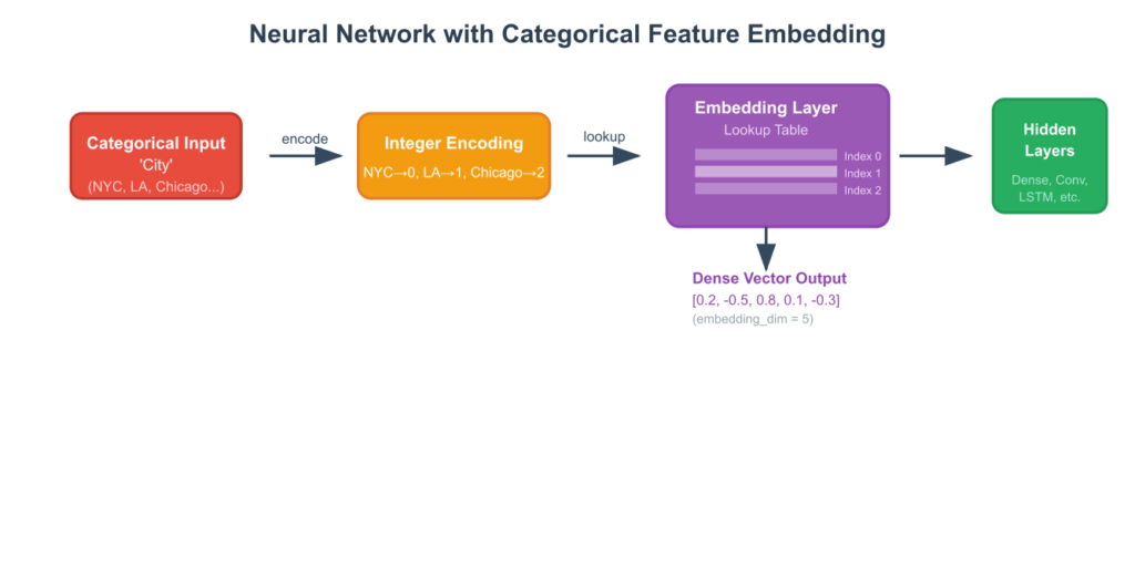
A more advanced and flexible approach, originating from the field of Natural Language Processing (NLP), is the use of entity embeddings. While a full treatment is beyond the scope of this chapter, it’s important to introduce the concept. Instead of using a fixed, rule-based encoding, embeddings learn a dense vector representation for each category during the model training process itself.
This is typically done using a neural network. The categorical feature is first integer-encoded. Then, an “embedding layer” in the network acts as a lookup table, mapping each integer to a dense vector of a predefined size (e.g., 10, 50, or 100 dimensions). The values in these vectors are initialized randomly and are then updated via backpropagation during training, just like the other weights in the network. The network learns to place categories that have a similar effect on the target variable close to each other in the multi-dimensional embedding space.
For example, in a movie recommendation system, the embeddings for ‘Action’ and ‘Sci-Fi’ might end up being closer together than the embeddings for ‘Action’ and ‘Romance’, because users who like action films often also like sci-fi films. This learned representation captures nuanced relationships between categories in a way that fixed encoding schemes cannot. It is a powerful method for high-cardinality data and is the de facto standard in modern deep learning applications involving categorical features.
Categorical Encoding Strategy Comparison
| Technique | Data Type | Pros | Cons | Best For |
|---|---|---|---|---|
| Ordinal Encoding | Ordinal | – Simple & efficient – Preserves order – Low dimensionality |
– Introduces artificial magnitude – Not for nominal data |
Features with clear, intrinsic ranking like ‘Low’, ‘Medium’, ‘High’. |
| One-Hot Encoding | Nominal | – No order assumption – Works well with linear models – Interpretable |
– Curse of Dimensionality – Inefficient for high cardinality |
Low-cardinality nominal features like ‘Color’ or ‘Department’. |
| Target Encoding | Nominal (High-Cardinality) | – Creates a single, powerful feature – Avoids high dimensionality – Captures predictive value |
– High risk of data leakage – Requires careful regularization – Less interpretable |
High-cardinality features like ‘ZIP Code’ or ‘user_id’, especially with tree-based models. |
| Entity Embeddings | Nominal (High-Cardinality) | – Learns semantic relationships – Creates dense, rich features – Handles complex interactions |
– Requires a neural network – Computationally intensive – Black-box nature |
Deep learning applications where nuanced relationships between categories are important (e.g., recommendation systems). |
Practical Examples and Implementation
Theory provides the foundation, but practical implementation solidifies understanding. This section translates the concepts of ordinal, one-hot, and target encoding into executable Python code, using standard data science libraries. We will demonstrate how to apply these techniques, visualize their effects, and solve computational exercises to reinforce the learning process.
Mathematical Concept Implementation
We’ll use pandas for data manipulation and scikit-learn for most encoding tasks. For target encoding, we’ll also use the category_encoders library, which provides a robust, production-ready implementation.
Let’s start by creating a sample dataset that includes ordinal, low-cardinality nominal, and high-cardinality nominal features.
import pandas as pd
import numpy as np

# Create a sample DataFrame
data = {
    'education_level': ['High School', 'Masters', 'Bachelors', 'PhD', 'Bachelors', 'Masters', 'High School'],
    'city': ['New York', 'London', 'Tokyo', 'London', 'New York', 'Tokyo', 'London'],
    'product_id': ['P101', 'P202', 'P303', 'P101', 'P202', 'P404', 'P303'],
    'target': [50, 95, 80, 75, 65, 85, 70] # A continuous target for regression
}
df = pd.DataFrame(data)

print("Original DataFrame:")
print(df)
Outputs:
Original DataFrame:
  education_level      city product_id  target
0     High School  New York       P101      50
1         Masters    London       P202      95
2       Bachelors     Tokyo       P303      80
3             PhD    London       P101      75
4       Bachelors  New York       P202      65
5         Masters     Tokyo       P404      85
6     High School    London       P303      70
Ordinal Encoding Implementation
For the education_level feature, there is a clear order. We can implement ordinal encoding manually or with scikit-learn‘s OrdinalEncoder.
from sklearn.preprocessing import OrdinalEncoder

# Define the explicit order of categories
education_order = ['High School', 'Bachelors', 'Masters', 'PhD']

# Initialize the encoder with the specified order
# The categories parameter is crucial for ensuring the correct mapping
ordinal_encoder = OrdinalEncoder(categories=[education_order])

# Apply the encoder
# Scikit-learn estimators expect a 2D array, so we use [['education_level']]
df['education_ordinal'] = ordinal_encoder.fit_transform(df[['education_level']])

print("\nDataFrame with Ordinal Encoding:")
print(df[['education_level', 'education_ordinal']])
Outputs:
DataFrame with Ordinal Encoding:
  education_level  education_ordinal
0     High School                0.0
1         Masters                2.0
2       Bachelors                1.0
3             PhD                3.0
4       Bachelors                1.0
5         Masters                2.0
6     High School                0.0
The code correctly maps the ordered categories to integers \(0, 1, 2, 3\), preserving the inherent ranking.
One-Hot Encoding Implementation
The city feature is nominal and has low cardinality, making it a perfect candidate for OHE. We can use pandas.get_dummies for a quick implementation or sklearn.preprocessing.OneHotEncoder for integration into a machine learning pipeline.
from sklearn.preprocessing import OneHotEncoder

# Using scikit-learn's OneHotEncoder
ohe = OneHotEncoder(sparse_output=False, handle_unknown='ignore')

# Fit and transform the 'city' column
# The output is a NumPy array of the new columns
city_encoded = ohe.fit_transform(df[['city']])

# Create a new DataFrame with the encoded columns
# Use get_feature_names_out() to get meaningful column names
ohe_df = pd.DataFrame(city_encoded, columns=ohe.get_feature_names_out(['city']))

# Concatenate with the original DataFrame
df_ohe = pd.concat([df.reset_index(drop=True), ohe_df], axis=1)

print("\nDataFrame with One-Hot Encoding:")
print(df_ohe[['city', 'city_London', 'city_New York', 'city_Tokyo']])
Outputs:
DataFrame with One-Hot Encoding:
       city  city_London  city_New York  city_Tokyo
0  New York          0.0            1.0         0.0
1    London          1.0            0.0         0.0
2     Tokyo          0.0            0.0         1.0
3    London          1.0            0.0         0.0
4  New York          0.0            1.0         0.0
5     Tokyo          0.0            0.0         1.0
6    London          1.0            0.0         0.0
This demonstrates how the single city column is expanded into three binary features, removing any artificial ordering. The handle_unknown='ignore' parameter is important for production systems; if a new city appears in the test data, it will be encoded as all zeros without throwing an error.
AI/ML Application Examples
Let’s now tackle the high-cardinality product_id feature using Target Encoding. This is where we need to be careful about data leakage. A production-grade implementation would use a cross-validation scheme. For simplicity here, we will use the category_encoders library which handles much of the complexity, including smoothing.
# Ensure you have the library installed: pip install category_encoders
import category_encoders as ce

# Initialize the TargetEncoder
# The smoothing parameter helps prevent overfitting to rare categories
target_encoder = ce.TargetEncoder(cols=['product_id'], smoothing=5.0)

# Fit and transform the data
# Note: you provide both X (features) and y (target) to this encoder
df['product_id_target'] = target_encoder.fit_transform(df['product_id'], df['target'])

print("\nDataFrame with Target Encoding:")
print(df[['product_id', 'target', 'product_id_target']].sort_values('product_id'))
Outputs:
DataFrame with Target Encoding:
  product_id  target  product_id_target
0       P101      50          73.972250
3       P101      75          73.972250
1       P202      95          74.437697
4       P202      65          74.437697
2       P303      80          74.304712
6       P303      70          74.304712
5       P404      85          74.520156
Notice how the encoder calculates the mean of the target for each product_id. For example, P101 appears with targets 50 and 75, so its encoding is related to the mean (62.5). The smoothing parameter adjusts this value based on the global target mean to make the encoding for rare categories more robust. This single new feature, product_id_target, now contains rich information about the predictive power of each product ID.
Visualization and Interactive Examples
Visualizing the result of encoding can provide valuable insights. Let’s visualize the relationship between our new target-encoded feature and the actual target. A strong positive correlation is expected by design.
import matplotlib.pyplot as plt
import seaborn as sns

plt.style.use('seaborn-v0_8-whitegrid')
fig, ax = plt.subplots(figsize=(8, 6))

sns.scatterplot(data=df, x='product_id_target', y='target', hue='product_id', s=200, ax=ax)
ax.set_title('Target vs. Target-Encoded Feature', fontsize=16)
ax.set_xlabel('Target-Encoded Product ID', fontsize=12)
ax.set_ylabel('Actual Target Value', fontsize=12)
plt.legend(title='Product ID')
plt.show()
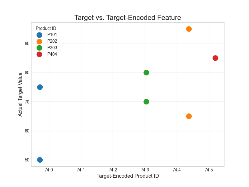
The plot clearly shows that the target-encoded feature effectively captures the predictive signal from the product_id category. Higher encoded values correspond to higher target values, creating a powerful continuous feature for a model to learn from.
Computational Exercises
To solidify your understanding, perform the following exercises.
Exercise 1: Manual Target Encoding Calculation
For the product_id ‘P303’, manually calculate its target encoding without smoothing.
- Step 1: Identify all rows where
product_idis ‘P303’. - Step 2: Find the corresponding
targetvalues for these rows. - Step 3: Calculate the average of these target values.
- Solution: The target values are 80 and 70. The average is \((80 + 70) / 2 = 75\). This demonstrates the core logic of the algorithm.
Exercise 2: One-Hot Encoding with a Dropped Category
Modify the OneHotEncoder implementation to drop one of the categories (e.g., ‘Tokyo’) to create dummy variables. Use the drop=’first’ parameter.
- Objective: Understand how to prevent multicollinearity.
- Implementation:
ohe_dropped = OneHotEncoder(sparse_output=False, drop='first')
city_encoded_dropped = ohe_dropped.fit_transform(df[['city']])
ohe_dropped_df = pd.DataFrame(city_encoded_dropped, columns=ohe_dropped.get_feature_names_out(['city']))
print("\nOHE with a Dropped Category:")
print(ohe_dropped_df)
The output will now have only two columns. A row with ‘Tokyo’ would be represented as \([0, 0]\) in these new columns.
Real-World Problem Applications
These encoding techniques are not just academic exercises; they are applied daily to solve real business problems.
- Computer Vision (Object Detection): While the image itself is numerical, the labels (‘cat’, ‘dog’, ‘car’) are categorical. In model training, these labels are often one-hot encoded to be used with a categorical cross-entropy loss function. The model outputs a probability vector, and the OHE vector serves as the ground truth.
- Natural Language Processing (NLP): Before the dominance of learned embeddings, traditional NLP models heavily relied on OHE for word representation (a “Bag of Words” model is essentially a massive OHE matrix). While modern techniques are more sophisticated, the underlying principle of converting discrete tokens into numerical vectors remains.
- Fraud Detection: A feature like ‘Merchant Category Code’ can have thousands of unique values. Target encoding is extremely effective here. By encoding the category with its historical fraud rate (the mean of a binary ‘is_fraud’ target), the model gains a powerful feature indicating the baseline risk associated with that type of merchant, without creating thousands of new columns.
Industry Applications and Case Studies
The choice of encoding strategy can have significant business implications, affecting everything from model performance to deployment costs. Here are several real-world case studies where categorical encoding plays a pivotal role.
- E-commerce Recommendation Engines:
- Use Case: Personalizing product recommendations on an e-commerce website. Features like
product_category,brand, anduser_segmentare highly predictive but categorical. - Implementation: High-cardinality features like
product_idoruser_idare often encoded using embedding techniques. A neural network learns dense vector representations for each user and product. The similarity between a user’s vector and a product’s vector can then be used to rank recommendations. For simpler models, features likebrandmight be target-encoded against a “purchase” or “click” binary target, effectively ranking brands by their popularity or conversion rate. - Business Impact: Improved recommendations lead directly to higher user engagement, conversion rates, and average order value. A 1% improvement in conversion can translate to millions of dollars in revenue for a large retailer.
- Use Case: Personalizing product recommendations on an e-commerce website. Features like
- Financial Fraud Detection:
- Use Case: Identifying fraudulent credit card transactions in real-time. Features include
transaction_type(e.g., ‘online’, ‘in-store’),merchant_id, andcountry_of_transaction. - Implementation Challenges:
merchant_idis extremely high-cardinality. One-Hot Encoding is computationally infeasible for a real-time system. Target encoding is a go-to solution, where eachmerchant_idis encoded with its historical fraud rate, heavily regularized to avoid overfitting. This provides a powerful risk score for each merchant. - Business Impact: Reducing false positives (legitimate transactions incorrectly flagged as fraud) improves customer experience, while catching more fraudulent transactions prevents direct financial losses. Efficient encoding is key to meeting low-latency requirements for real-time transaction approval.
- Use Case: Identifying fraudulent credit card transactions in real-time. Features include
- Predictive Maintenance in Manufacturing:
- Use Case: Predicting when a piece of industrial machinery will fail, based on sensor data and operational logs. Categorical features might include
machine_model,factory_location, anderror_code. - Implementation:
error_codecan be a high-cardinality feature. A combination of one-hot encoding for low-cardinality features likefactory_locationand target encoding forerror_code(using a “failure in next 24 hours” target) can be highly effective. The target-encoded error code essentially becomes a feature representing the historical failure probability associated with that specific error. - Business Impact: Proactively servicing machinery before it fails minimizes unplanned downtime, which is a massive source of cost and inefficiency in manufacturing. This leads to improved operational efficiency and reduced maintenance costs.
- Use Case: Predicting when a piece of industrial machinery will fail, based on sensor data and operational logs. Categorical features might include
Best Practices and Common Pitfalls
Effective categorical encoding requires more than just knowing the APIs; it demands a strategic approach that considers the data, the model, and the deployment context. Adhering to best practices and avoiding common pitfalls is crucial for building robust and high-performing AI systems.
%%{init: {'theme': 'base', 'themeVariables': { 'fontFamily': 'Open Sans'}}}%%
graph TD
    A[Start: Categorical Feature] --> B{Is there an<br>intrinsic order?};
    B -- Yes --> C[Ordinal Encoding];
    B -- No --> D{What is the<br>cardinality?};
    D -- Low <br> (e.g., < 50 cats) --> E[One-Hot Encoding];
    D -- High <br> (e.g., > 50 cats) --> F{What type of<br>model are you using?};
    F -- Tree-Based Models <br> (XGBoost, RF) --> G["Target Encoding<br><i>(Use CV to prevent leakage)</i>"];
    F -- Neural Networks --> H[Entity Embeddings];
    F -- Other/Unsure --> I[Consider Feature Hashing<br>or Grouping Rare Categories];
    C --> Z[End];
    E --> Z[End];
    G --> Z[End];
    H --> Z[End];
    I --> Z[End];

    %% Styling
    classDef startNode fill:#283044,stroke:#283044,stroke-width:2px,color:#ebf5ee;
    classDef endNode fill:#2d7a3d,stroke:#2d7a3d,stroke-width:2px,color:#ebf5ee;
    classDef decisionNode fill:#f39c12,stroke:#f39c12,stroke-width:1px,color:#283044;
    classDef processNode fill:#78a1bb,stroke:#78a1bb,stroke-width:1px,color:#283044;
    classDef modelNode fill:#e74c3c,stroke:#e74c3c,stroke-width:1px,color:#ebf5ee;
    classDef cautionNode fill:#f1c40f,stroke:#f1c40f,stroke-width:1px,color:#283044;

    class A startNode;
    class Z endNode;
    class B,D,F decisionNode;
    class C,E processNode;
    class G,H modelNode;
    class I cautionNode;
- Match Encoding to Model Type: The optimal encoding strategy often depends on the machine learning algorithm being used.
- Linear Models & Neural Networks: These models generally perform best with One-Hot Encoding because it creates independent features, which aligns with their assumptions. They struggle to extract value from a single column of ordinally encoded nominal data.
- Tree-Based Models (Random Forest, Gradient Boosting): These models are more flexible. They can handle ordinally encoded nominal data better than linear models because they partition the data based on thresholds (e.g.,
city_code < 3). However, OHE can still be beneficial. Target encoding is often extremely effective with tree-based models, as they are adept at finding optimal split points on the resulting continuous feature.
- Handle Unseen Categories in Production: This is a critical production issue. Your trained encoder has only seen the categories present in the training data. What happens when a new category appears in the data you need to predict on?
- Pitfall: The default behavior of many encoders is to throw an error, which would crash a production pipeline.
- Best Practice: Explicitly plan for this.
sklearn.OneHotEncoderhas ahandle_unknown='ignore'parameter, which encodes the new category as a vector of all zeros. For target encoding, new categories can be mapped to the global mean of the target. This ensures the system is robust and does not fail on new, legitimate data.
- Beware of Data Leakage with Target Encoding: As emphasized previously, this is the single biggest pitfall of target encoding.
- Pitfall: Calculating encodings on the entire dataset and then splitting into training and validation sets. This leaks information from the validation target into the training features, leading to overly optimistic performance metrics and a model that fails to generalize.
- Best Practice: Always use a robust validation scheme. The gold standard is to compute target encodings within each fold of a cross-validation loop, using only the data from the other folds. For a final model, you compute encodings on the full training set and apply them to the test set.
- Manage High Cardinality Intelligently: Don’t blindly apply One-Hot Encoding to features with thousands of categories.
- Pitfall: Creating a massive, sparse feature matrix that exhausts memory and dramatically slows down training.
- Best Practice: Consider alternatives. If a feature has a long-tail distribution (many categories appear very infrequently), group rare categories into a single “Other” category before encoding. For truly high-cardinality features, prioritize Target Encoding or Entity Embeddings.
- Do Not Ordinally Encode Nominal Data: This fundamental error introduces artificial relationships that can confuse the model and degrade performance. Always question if there is a true, undeniable order to the categories before choosing Ordinal Encoding.
Hands-on Exercises
These exercises are designed to build upon the chapter’s concepts, progressing from foundational implementation to more complex, real-world scenarios.
- Feature Engineering for a Customer Churn Dataset:
- Objective: Apply various encoding techniques to a realistic dataset and evaluate their impact.
- Dataset: Create a mock customer churn dataset with features like
gender(nominal, low-cardinality),subscription_plan(‘Basic’, ‘Standard’, ‘Premium’ – ordinal),country(nominal, high-cardinality), and a binarychurntarget. - Tasks:
- Apply One-Hot Encoding to the
gendercolumn. - Apply Ordinal Encoding to the
subscription_plancolumn, ensuring the correct order is specified. - Apply Target Encoding to the
countrycolumn using thechurntarget. - Train a simple logistic regression model on the dataset using each encoding strategy in isolation and compare their validation accuracy. Discuss why some encodings might work better than others for this model.
- Apply One-Hot Encoding to the
- Building a Robust Preprocessing Pipeline:
- Objective: Use
scikit-learn‘sPipelineandColumnTransformerto build a reproducible and robust preprocessing workflow. - Tasks:
- Use the dataset from Exercise 1.
- Create a
ColumnTransformerthat appliesOneHotEncoderto the nominal columns andOrdinalEncoderto the ordinal columns simultaneously. - Encapsulate this
ColumnTransformerand a machine learning model (e.g.,RandomForestClassifier) within aPipelineobject. - Train the entire pipeline on your data. This is the standard practice for preventing data leakage and ensuring that the same transformations are applied consistently to training and testing data.
- Bonus: Add a step to the pipeline to handle missing values before encoding.
- Objective: Use
- Investigating the Impact of Smoothing in Target Encoding:
- Objective: Understand how the
smoothingparameter in Target Encoding affects model robustness. - Tasks:
- Create a synthetic dataset where some categories are very rare but are perfectly correlated with the target (e.g., a category appears once, and the target is 1).
- Apply Target Encoding twice: once with a very low smoothing value (e.g.,
smoothing=1) and once with a higher value (e.g.,smoothing=50). - Observe the encoded values for the rare categories in both cases.
- Discuss how high smoothing helps prevent the model from overfitting to these rare, noisy categories by pulling their encoded value closer to the global average.
- Objective: Understand how the
Tools and Technologies
The practical implementation of categorical encoding relies on a mature ecosystem of Python libraries. Mastery of these tools is essential for any AI engineer.
- Pandas: The cornerstone of data manipulation in Python. It is used for loading, cleaning, and exploring data. Its
get_dummies()function provides a quick and easy way to perform one-hot encoding, which is excellent for initial exploratory analysis. - Scikit-learn: The fundamental machine learning library in Python. Its
preprocessingmodule contains robust, pipeline-compatible implementations of encoders likeOrdinalEncoderandOneHotEncoder. Using these classes is the recommended practice for building production-ready models, as they integrate seamlessly withPipelineandColumnTransformerobjects, ensuring proper data handling and preventing leakage. Version 1.0 and later offer consistent and powerful features. - Category Encoders: This is a specialized, open-source library dedicated to categorical variable encoding. It provides scikit-learn compatible implementations of numerous advanced techniques not found in the base scikit-learn library, including
TargetEncoder,CatBoostEncoder, andJamesSteinEncoder. It is the go-to tool for implementing sophisticated strategies like target encoding in a robust and well-tested manner. - NumPy: The foundational library for numerical computation in Python. While you may not use it directly for encoding, it underpins the operations of all the other libraries. The arrays generated by scikit-learn encoders are NumPy arrays.
- Matplotlib & Seaborn: These are the primary libraries for data visualization. They are crucial for the exploratory data analysis (EDA) step, where you investigate the distributions of your categorical variables and their relationship with the target, which helps inform your choice of encoding strategy.
Summary
This chapter provided a comprehensive exploration of categorical data encoding, a critical step in preparing data for machine learning models. We established the fundamental principles and moved through progressively advanced techniques.
- Key Concepts: We learned that categorical data must be converted into a numerical format for algorithms to process. We distinguished between nominal (no order) and ordinal (inherent order) data, a distinction that governs the choice of encoding method.
- Foundational Techniques: We implemented Ordinal Encoding for data with a natural ranking and One-Hot Encoding for nominal data, noting its major drawback of increasing dimensionality.
- Advanced Strategies: To handle high-cardinality features, we explored Target Encoding, a powerful method that uses the target variable to create a dense, predictive feature. We emphasized the critical importance of using regularization techniques like smoothing and cross-validation to prevent data leakage and overfitting.
- Practical Skills: Through Python examples using
pandas,scikit-learn, andcategory_encoders, you have gained the practical skills to implement these strategies within robust, reproducible machine learning pipelines. - Real-World Applicability: The techniques covered are not theoretical; they are essential tools used in production AI systems across industries like finance, e-commerce, and manufacturing to unlock the value in non-numeric data.
Further Reading and Resources
- Scikit-learn Documentation on Preprocessing: The official documentation is the definitive source for understanding the parameters and usage of
OrdinalEncoder,OneHotEncoder, and other related tools. (https://scikit-learn.org/stable/modules/preprocessing.html) - Category Encoders Library Documentation: An essential resource for implementing a wide variety of advanced encoding techniques, including Target Encoding. (https://contrib.scikit-learn.org/category_encoders/)
- “A Preprocessing Pipeline for Production” by an MLOps Expert: A detailed blog post or tutorial from a reputable source like the Google AI Blog or Netflix TechBlog that walks through building a production-grade feature engineering pipeline, emphasizing robustness and handling unseen values.
- “Entity Embeddings of Categorical Variables” (Paper): The 2016 paper by Guo and Berkhahn that popularized the use of learned embeddings for categorical data in the context of tabular data competitions and applications. (https://arxiv.org/abs/1604.06737)
- “Feature Engineering for Machine Learning” by Alice Zheng & Amanda Casari: This O’Reilly book provides a deep, practical dive into many feature engineering topics, with excellent chapters on handling categorical variables.
- Kaggle Notebooks: Exploring winning solutions from Kaggle competitions is an excellent way to see how world-class data scientists use advanced encoding techniques in practice. Search for notebooks on competitions with tabular data.
Glossary of Terms
- Categorical Variable: A variable that can take on one of a limited, and usually fixed, number of possible values, assigning each individual or other unit of observation to a particular group or nominal category on the basis of some qualitative property.
- Cardinality: The number of unique values in a categorical feature. ‘Low cardinality’ means few unique values; ‘high cardinality’ means many unique values.
- Curse of Dimensionality: A term describing the various problems that arise when working with data in high-dimensional spaces, including data sparsity and increased computational complexity.
- Data Leakage: The introduction of information into a model’s training process that would not be available at prediction time. This leads to an overly optimistic evaluation of model performance. Target encoding without proper validation is a classic cause of data leakage.
- Dummy Variables: The binary features created by One-Hot Encoding. The practice of dropping one of the \(k\) columns to create \(k-1\) features is known as creating dummy variables.
- Entity Embedding: A learned, dense, low-dimensional vector representation of a category. The relationships (e.g., distance and direction) between vectors in the embedding space capture the semantic relationships between the categories.
- Nominal Variable: A categorical variable where the categories have no intrinsic order or ranking (e.g., ‘City’).
- One-Hot Encoding (OHE): A process of converting a categorical variable into a set of binary features (0s and 1s), where each new feature represents a unique category.
- Ordinal Variable: A categorical variable where the categories have a clear, inherent order or ranking (e.g., ‘Education Level’).
- Target Encoding (Mean Encoding): A technique where each category is replaced with the mean of the target variable for all samples belonging to that category. Requires careful regularization to prevent overfitting.
