
Chapter 15: Bayesian Statistics and Probability in Machine Learning
Chapter Objectives
Upon completing this chapter, you will be able to:
- Understand the foundational principles of Bayesian probability and distinguish it from the Frequentist approach.
- Implement Bayes’ theorem to update beliefs and perform statistical inference using prior, posterior, likelihood, and evidence.
- Analyze the role of prior and posterior distributions in probabilistic modeling and uncertainty quantification.
- Design and build Bayesian models for tasks like classification and regression using modern Python libraries.
- Optimize Bayesian models by selecting appropriate priors and utilizing computational techniques like Markov Chain Monte Carlo (MCMC).
- Deploy probabilistic models with an understanding of their performance characteristics, benefits, and limitations in production environments.
Introduction
In the landscape of modern AI engineering, the ability to quantify uncertainty is not merely a feature—it is a cornerstone of building robust, reliable, and trustworthy systems. While many machine learning models provide point estimates (a single “best” prediction), they often fail to communicate their confidence. A model might predict a 95% probability of a financial transaction being fraudulent, but is it 95% certain, or is it merely its best guess in a highly uncertain scenario? Answering this question is the domain of Bayesian statistics. This chapter introduces a different paradigm for reasoning under uncertainty, shifting from the classical Frequentist view of probability as a long-run frequency to the Bayesian perspective of probability as a degree of belief.
This approach, rooted in the 18th-century work of Thomas Bayes, provides a powerful mathematical framework for updating our beliefs in the face of new evidence. For the AI engineer, this translates into tangible benefits: models that can express uncertainty, systems that can learn incrementally from new data streams, and frameworks for incorporating domain knowledge directly into the learning process. From building self-driving car perception systems that must reason about the likelihood of an object being a pedestrian to developing medical diagnostic tools that quantify the probability of a disease, Bayesian methods are indispensable. In this chapter, we will build a strong theoretical foundation in Bayesian inference, explore its mathematical underpinnings, and translate that theory into practice by implementing probabilistic models that are not only accurate but also aware of their own limitations.
Technical Background
The transition from deterministic predictions to probabilistic reasoning represents a significant leap in the sophistication of AI systems. At the heart of this leap lies the Bayesian framework, which provides a principled and coherent language for managing uncertainty. This section delves into the core concepts of Bayesian statistics, tracing their historical development and establishing the mathematical and architectural principles that underpin their application in modern machine learning.
Fundamental Concepts and Definitions
To navigate the world of probabilistic machine learning, we must first establish a firm grasp of its core lexicon and mathematical machinery. The Bayesian viewpoint is fundamentally about belief updating. It posits that our understanding of the world is never static; it is a dynamic state of knowledge that evolves as we gather more data. This contrasts sharply with the Frequentist approach, which treats parameters as fixed, unknown constants and probability as the long-run frequency of an event over repeated trials. For a Bayesian, a parameter is a random variable about which we can have beliefs, and probability is a measure of the plausibility of a statement given our current state of knowledge.
| Aspect | Bayesian Approach | Frequentist Approach |
|---|---|---|
| Definition of Probability | A degree of belief or confidence in a statement, which can be updated with new evidence. | The long-run frequency of an event over many repeated trials. |
| Model Parameters | Considered random variables about which we can have beliefs, described by probability distributions. | Considered fixed, unknown constants that we aim to estimate. |
| Core Output | A full posterior probability distribution for the parameters, quantifying uncertainty. | A single point estimate for parameters and confidence intervals based on sampling distributions. |
| Role of Prior Knowledge | Formally incorporated into the model via a prior distribution. | Generally avoided in the formal model, though it influences model choice and design. |
| Key Question Answered | “Given the data, what is the probability that the parameter is in a certain range?” (e.g., Credible Interval) | “If we repeated the experiment many times, what percentage of confidence intervals would contain the true parameter?” |
Core Terminology and Mathematical Foundations
The cornerstone of Bayesian statistics is Bayes’ Theorem. It is an elegant and remarkably powerful formula that describes how to update the probability of a hypothesis based on new evidence. Mathematically, it is expressed as: \[P(\theta|D) = \frac{P(D|\theta)P(\theta)}{P(D)}\]
Let’s dissect this equation, as every component is critical to the Bayesian workflow:
- Posterior Probability \( P(\theta | D) \): This is the probability of our hypothesis \( \theta \) after observing the data \( D \). It represents our updated belief. This is the quantity we typically want to compute. The term “posterior” signifies that it is post-data.
- Likelihood \( P(D | \theta) \): This is the probability of observing the data \( D \) given that our hypothesis \( \theta \) is true. It is a function of \( \theta \) and is the component that connects our model to the data. In machine learning, this is often defined by the model we choose (e.g., a linear regression model assumes the data is generated from a line with some noise).
- Prior Probability \( P(\theta) \): This is the probability of our hypothesis \( \theta \) before observing any data. It represents our initial belief or knowledge about the parameter. This is a key feature of Bayesian methods, allowing us to incorporate domain expertise or previous findings directly into the model. The choice of prior can significantly influence the posterior, especially with limited data.
- Evidence (or Marginal Likelihood) \( P(D) \): This is the total probability of observing the data, averaged over all possible hypotheses. It is calculated by integrating (or summing) the product of the likelihood and the prior over the entire parameter space: \[P(D) = \int P(D | \theta) P(\theta) , d\theta\]. The evidence serves as a normalization constant, ensuring that the posterior probability distribution integrates to 1.
Because the evidence \( P(D) \) can be computationally intractable to calculate, especially for complex models with many parameters, it is often treated as a constant. This leads to a more practical, proportional form of Bayes’ rule: \[P(\theta|D) \propto P(D|\theta)P(\theta)\]
This relationship—Posterior \( \propto \) Likelihood \( \times \) Prior—is the engine of Bayesian inference. It tells us precisely how to combine our prior beliefs with the evidence from the data to arrive at an updated, posterior belief.
graph TD
    subgraph "Bayesian Inference Engine"
        direction LR
        A[("<b>Prior Belief</b><br><i>P(θ)</i><br>Initial knowledge about parameters")]
        B[("<b>Likelihood</b><br><i>P(D|θ)</i><br>How well parameters explain the data")]
        C{"<b>Bayes' Rule</b><br>Posterior ∝ Likelihood × Prior"}
        D[("<b>Posterior Belief</b><br><i>P(θ|D)</i><br>Updated knowledge after seeing data")]

        A -- "Prior Distribution" --> C
        B -- "Data Evidence" --> C
        C -- "Computes" --> D
    end

    style A fill:#9b59b6,stroke:#9b59b6,stroke-width:2px,color:#ebf5ee
    style B fill:#78a1bb,stroke:#78a1bb,stroke-width:1px,color:#283044
    style C fill:#f39c12,stroke:#f39c12,stroke-width:1px,color:#283044
    style D fill:#2d7a3d,stroke:#2d7a3d,stroke-width:2px,color:#ebf5ee

Historical Development and Evolution
The theorem that now bears Thomas Bayes’ name was published posthumously in 1763 by his friend Richard Price. For nearly two centuries, it remained a mathematical curiosity, overshadowed by the burgeoning Frequentist school of thought championed by figures like Ronald Fisher. The Frequentist view, with its emphasis on objectivity and long-run frequencies, was more easily applied to the scientific and industrial problems of the era.
The Bayesian resurgence began in the mid-20th century, fueled by the work of Harold Jeffreys and Leonard “Jimmie” Savage, who championed its philosophical coherence. However, the primary obstacle to its widespread adoption was computational. Calculating the evidence term \( P(D) \) required solving complex, high-dimensional integrals, a task that was impossible for all but the simplest of models. The turning point came with the advent of powerful computers and the development of Markov Chain Monte Carlo (MCMC) methods in the 1980s and 1990s. Algorithms like the Metropolis-Hastings algorithm and the Gibbs sampler provided a way to approximate the posterior distribution \( P(\theta | D) \) without calculating the evidence directly. Instead of solving the integral, these methods draw samples from the posterior distribution, allowing us to characterize it empirically. This computational breakthrough unlocked the practical application of Bayesian methods to complex, real-world problems, paving the way for their integration into modern machine learning.
Technical Architecture and Design Principles
Applying Bayesian principles in a machine learning context involves more than just plugging numbers into a formula. It requires a shift in architectural thinking, from designing models that produce single-point estimates to building systems that manage and propagate distributions of belief. This probabilistic approach influences everything from model selection to deployment and monitoring.
System Components and Interactions
A typical Bayesian machine learning system can be broken down into several key components that interact to learn from data and generate predictions.
- Prior Distribution Selection: This is the first step in defining a Bayesian model. The choice of prior is a powerful mechanism for injecting domain knowledge into the model. A non-informative prior (e.g., a uniform distribution over a wide range) is used when we have little initial knowledge and want the data to speak for itself. An informative prior (e.g., a normal distribution centered on a known value) is used when we have strong pre-existing information. Conjugate priors are a special class of priors that, when combined with a given likelihood, result in a posterior distribution from the same family, simplifying the math considerably. For example, the Beta distribution is the conjugate prior for the Bernoulli likelihood.
- Likelihood Function Definition: This component defines the generative process of the data. It’s the statistical model we assume is responsible for creating the observed data, given a set of parameters \( \theta \). For a regression problem, the likelihood might be a normal distribution centered around the output of a linear equation. For classification, it might be a Bernoulli or Categorical distribution. The choice of likelihood is a critical modeling decision that reflects our assumptions about the data-generating process.
- Inference Engine: This is the computational core of the system. Its job is to combine the prior and the likelihood to compute the posterior distribution of the parameters. For simple models with conjugate priors, this can be an analytical calculation. For most real-world models, however, this requires sophisticated approximation techniques. The dominant methods are Markov Chain Monte Carlo (MCMC), which includes algorithms like Metropolis-Hastings and No-U-Turn Sampler (NUTS), and Variational Inference (VI), which reframes the inference problem as an optimization problem, often providing a faster but less exact approximation.
- Posterior Predictive Distribution: Once we have the posterior distribution of the parameters \( P(\theta | D) \), we can make predictions for new, unseen data points \( x_{new} \). A simple approach would be to take a point estimate from the posterior (like the mean or median) and use that for prediction. However, the truly Bayesian approach is to calculate the posterior predictive distribution, which averages the predictions over all possible parameter values, weighted by their posterior probability: \[P(y_{\text{new}}|x_{\text{new}},D) = \int P(y_{\text{new}}|x_{\text{new}},\theta)P(\theta|D) , d\theta\]. This represents the prediction for new data \(y_{\text{new}}\) given input \(x_{\text{new}}\) and observed data \(D\). This process naturally incorporates parameter uncertainty into our predictions. A wide posterior predictive distribution indicates high uncertainty in the prediction.
graph TD
    A("<b>Start: Define Problem</b>") --> B{"<b>Choose Priors P(θ)</b><br><i>Incorporate domain knowledge.<br>Perform prior predictive checks.</i>"};
    B --> C["<b>Define Likelihood P(D|θ)</b><br><i>Select a statistical model<br>that reflects the data<br>generating process.</i>"];
    C --> D[("<b>Collect & Preprocess Data D</b>")];
    D --> E{"<b>Perform Inference</b><br><i>Combine prior and likelihood<br>to compute the posterior P(θ|D)</i>"};
    E -- "MCMC (e.g., NUTS)" --> F["<b>Posterior Distribution P(θ|D)</b>"];
    E -- "Variational Inference (VI)" --> F;
    F --> G{"<b>Analyze Posterior</b><br><i>Check MCMC convergence (R-hat, ESS).<br>Visualize distributions.<br>Calculate credible intervals.</i>"};
    G --> H["<b>Perform Posterior<br>Predictive Checks</b><br><i>Simulate data from the model.<br>Compare to observed data.</i>"];
    H --> I{<b>Model adequate?</b>};
    I -- "No --> Revise Model" --> B;
    I -- "Yes -->" --> J[("<b>Generate Predictions</b><br><i>Use posterior predictive distribution<br>to quantify prediction uncertainty.</i>")];
    J --> K(("<b>End: Deploy & Monitor</b>"));

    classDef start fill:#283044,stroke:#283044,stroke-width:2px,color:#ebf5ee;
    classDef endo fill:#2d7a3d,stroke:#2d7a3d,stroke-width:2px,color:#ebf5ee;
    classDef process fill:#78a1bb,stroke:#78a1bb,stroke-width:1px,color:#283044;
    classDef decision fill:#f39c12,stroke:#f39c12,stroke-width:1px,color:#283044;
    classDef data fill:#9b59b6,stroke:#9b59b6,stroke-width:1px,color:#ebf5ee;
    classDef model fill:#e74c3c,stroke:#e74c3c,stroke-width:1px,color:#ebf5ee;
    classDef warning fill:#f1c40f,stroke:#f1c40f,stroke-width:1px,color:#283044;

    class A,K start;
    class C,F,H,J process;
    class B,E,G,I decision;
    class D data;
Design Patterns and Best Practices
Building robust Bayesian systems requires adherence to certain design patterns. One of the most important is the iterative modeling workflow. This involves starting with a simple model, checking its fit to the data, and gradually increasing its complexity. Prior predictive checks are a crucial part of this process, where we generate data from the prior distribution before seeing the actual data to ensure our priors lead to reasonable outcomes. Similarly, posterior predictive checks involve generating replicated datasets from the fitted model and comparing them to the observed data to diagnose model misfit.
Another key practice is sensitivity analysis. How much does our posterior conclusion depend on our choice of prior? By running the model with different priors (e.g., one informative, one non-informative), we can assess the robustness of our findings. If the posterior changes dramatically, it tells us the data is not very informative, and our prior beliefs are highly influential. If the posterior remains stable, it suggests the data is strong enough to override different initial beliefs. This transparency about the influence of assumptions is a major strength of the Bayesian approach.
Tip: When starting a new Bayesian analysis, begin with the simplest possible model. A simple model that you understand well is far more valuable than a complex model that is a black box. Use posterior predictive checks to identify where your model fails, and let those failures guide your next iteration of model improvement.
Advanced Topics and Modern Approaches
As the scale of data and the complexity of models have grown, so too have the techniques for performing Bayesian inference. The field is vibrant, with ongoing research into making Bayesian methods more scalable, automated, and applicable to the challenges of modern AI, such as deep learning.
Current Research Directions
A major frontier in Bayesian research is the intersection with deep learning. Bayesian Neural Networks (BNNs) replace the single-weight values of a standard neural network with distributions. Instead of learning a single point estimate for each weight, a BNN learns a posterior distribution over its weights. This allows the network to quantify its uncertainty, providing more reliable predictions, especially for out-of-distribution inputs. Training these models is computationally intensive, and techniques like Variational Inference are essential. The Bayes-by-backprop algorithm is a popular method for training BNNs by applying VI principles to the network’s weights.
Another active area is probabilistic programming. Probabilistic Programming Languages (PPLs) like Stan, PyMC, and Pyro allow developers to define complex Bayesian models using a concise, high-level syntax. The PPL automatically handles the underlying inference, compiling the model definition into an efficient computational backend that runs MCMC or VI. This abstraction allows practitioners to focus on model design rather than the intricate details of the inference algorithm, democratizing access to powerful Bayesian techniques.

Performance Optimization and Scalability
The primary bottleneck for Bayesian methods remains computational cost. Standard MCMC algorithms can be prohibitively slow for large datasets and high-dimensional models. This has spurred the development of more scalable inference techniques.
Variational Inference (VI) has emerged as a leading alternative to MCMC for large-scale applications. VI reframes inference as an optimization problem. It proposes a simpler, parameterized family of distributions (e.g., a multivariate normal distribution) and then tunes the parameters of this family to find the distribution that is “closest” to the true posterior. The measure of closeness is typically the Kullback-Leibler (KL) divergence. While VI is often much faster than MCMC, it comes with a trade-off: it provides an approximation to the posterior, which may not capture its full shape, and it tends to underestimate the variance of the posterior.
For MCMC, significant performance gains have been achieved through Hamiltonian Monte Carlo (HMC) and its adaptive variant, the No-U-Turn Sampler (NUTS). These algorithms, used by default in Stan and PyMC, explore the parameter space much more efficiently than simpler random-walk methods, especially in high dimensions. They do this by introducing auxiliary momentum variables, borrowing concepts from Hamiltonian physics to propose distant, high-probability states, leading to faster convergence and less correlated samples. For massive datasets, methods like Stochastic Gradient Langevin Dynamics (SGLD) and Stochastic Variational Inference (SVI) adapt these algorithms to work with mini-batches of data, bridging the gap between Bayesian inference and the stochastic optimization techniques common in deep learning.
| Feature | Markov Chain Monte Carlo (MCMC) | Variational Inference (VI) |
|---|---|---|
| Core Idea | Approximates the posterior by drawing samples from it. Converges to the true posterior in the limit. | Frames inference as an optimization problem: finds the “closest” simple distribution to the true posterior. |
| Accuracy | Asymptotically exact. Provides a highly accurate approximation of the true posterior if run long enough. | Provides an approximation. Tends to underestimate posterior variance and may not capture complex shapes. |
| Speed | Can be very slow, especially for large datasets and high-dimensional models. Each step can be computationally intensive. | Often much faster than MCMC. More amenable to mini-batch updates (stochastic VI) and hardware acceleration. |
| Scalability | Scalability is a major challenge. Standard algorithms often require the full dataset at each step. | Excellent scalability. The method of choice for large-scale Bayesian deep learning. |
| When to Use | When accuracy is paramount and computational time is less of a constraint. For smaller to medium-sized problems. | For very large datasets or models where speed and scalability are critical, and an approximation is acceptable. |
| Example Algorithms | Metropolis-Hastings, Gibbs Sampling, Hamiltonian Monte Carlo (HMC), NUTS. | Automatic Differentiation Variational Inference (ADVI), Bayes-by-backprop. |
Practical Examples and Implementation
Theory provides the “what” and “why,” but practical implementation provides the “how.” This section translates the foundational concepts of Bayesian statistics into executable Python code. We will leverage standard scientific computing and machine learning libraries to build, analyze, and visualize Bayesian models, bridging the gap between abstract mathematics and concrete AI applications.
Mathematical Concept Implementation
Let’s start by implementing Bayes’ theorem for a simple, intuitive problem: coin flipping. Suppose we have a coin that might be biased. Our goal is to estimate its probability of landing heads, which we’ll call \( \theta \).
A Simple Bayesian Update
We’ll use Python and NumPy to perform a single Bayesian update.
- Prior: We’ll start with a non-informative prior: a uniform distribution between 0 and 1. This represents the belief that any value of \( \theta \) is equally likely before we see any data.
- Likelihood: The likelihood of our data (e.g., observing \( k \) heads in \( n \) flips) is given by the Binomial distribution: \[P(D|\theta) = \left(\begin{array}{c} n \ k \end{array}\right) \theta^k (1-\theta)^{n-k}\]
- Posterior: Since the Beta distribution is the conjugate prior for the Binomial likelihood, if we use a Beta distribution for the prior, our posterior will also be a Beta distribution. A uniform distribution is a special case of the Beta distribution: \( \text{Beta}(1, 1) \). If our prior is \( \text{Beta}(\alpha, \beta) \) and we observe \( k \) successes and \( n-k \) failures, our posterior is \( \text{Beta}(\alpha+k, \beta+n-k) \).
import numpy as np
import matplotlib.pyplot as plt
from scipy.stats import beta

# --- Parameters ---
# True probability of heads (we don't know this in a real scenario)
true_theta = 0.6
# Number of coin flips in our experiment
n_flips = 20
# Prior parameters (alpha=1, beta=1 for a uniform prior)
alpha_prior = 1
beta_prior = 1

# --- Simulate Data ---
# Generate some data by flipping the coin n_flips times
data = np.random.binomial(1, true_theta, n_flips)
num_heads = np.sum(data)
num_tails = n_flips - num_heads

print(f"Observed Data: {num_heads} heads and {num_tails} tails in {n_flips} flips.")

# --- Bayesian Update ---
# The posterior parameters are updated based on the data
alpha_posterior = alpha_prior + num_heads
beta_posterior = beta_prior + num_tails

# --- Visualization ---
x = np.linspace(0, 1, 1000)

# Prior distribution (Beta(1, 1) is uniform)
prior_pdf = beta.pdf(x, alpha_prior, beta_prior)

# Posterior distribution
posterior_pdf = beta.pdf(x, alpha_posterior, beta_posterior)

plt.style.use('seaborn-v0_8-whitegrid')
fig, ax = plt.subplots(figsize=(12, 7))

ax.plot(x, prior_pdf, label=f'Prior: Beta({alpha_prior}, {beta_prior})', linestyle='--', color='gray')
ax.plot(x, posterior_pdf, label=f'Posterior: Beta({alpha_posterior}, {beta_posterior})', color='blue', linewidth=2.5)

# Add a vertical line for the true value of theta for reference
ax.axvline(true_theta, color='red', linestyle=':', label=f'True θ = {true_theta}')

ax.set_xlabel('θ (Probability of Heads)', fontsize=14)
ax.set_ylabel('Probability Density', fontsize=14)
ax.set_title(f'Bayesian Inference for a Coin Flip ({n_flips} trials)', fontsize=16)
ax.legend(fontsize=12)
ax.fill_between(x, posterior_pdf, color='blue', alpha=0.1)
plt.show()

# --- Quantifying Uncertainty ---
# We can calculate a credible interval from the posterior
credible_interval = beta.interval(0.95, alpha_posterior, beta_posterior)
print(f"\n95% Credible Interval for θ: [{credible_interval[0]:.3f}, {credible_interval[1]:.3f}]")
posterior_mean = beta.mean(alpha_posterior, beta_posterior)
print(f"Posterior Mean (point estimate): {posterior_mean:.3f}")
Output:
Observed Data: 14 heads and 6 tails in 20 flips.

95% Credible Interval for θ: [0.478, 0.854]
Posterior Mean (point estimate): 0.682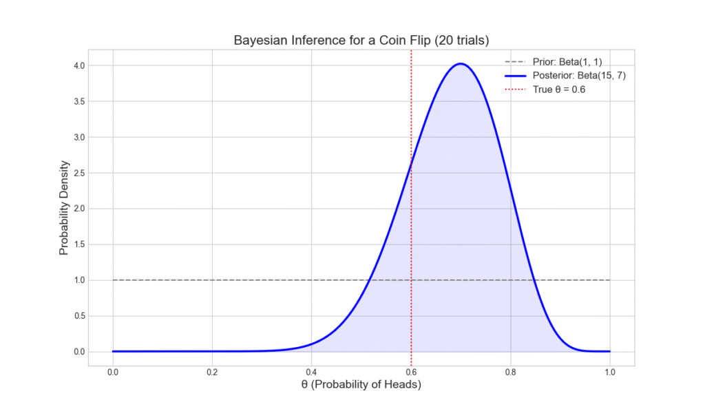
This example beautifully illustrates the core Bayesian mechanism. We started with a wide, uncertain prior. After observing data, we arrived at a much narrower posterior distribution, centered closer to the true value of \( \theta \). The 95% credible interval gives us a range of plausible values for the coin’s bias, directly quantifying our uncertainty.
AI/ML Application Examples
Now, let’s apply these concepts to a more traditional machine learning problem: Bayesian Linear Regression. Unlike standard linear regression which finds a single best-fit line (i.e., single values for the slope and intercept), Bayesian linear regression estimates the posterior distribution for the slope and intercept.
We’ll use the popular probabilistic programming library PyMC.
import pymc as pm
import numpy as np
import matplotlib.pyplot as plt
import arviz as az

# --- Generate Synthetic Data ---
np.random.seed(42)
true_slope = 2.5
true_intercept = -1.0
noise_std = 2.0

# Generate 50 data points
X = np.linspace(0, 10, 50)
y = true_intercept + true_slope * X + np.random.normal(0, noise_std, size=50)

# --- Define and Run the Bayesian Model ---
with pm.Model() as linear_model:
    # Priors for the model parameters
    # Using weakly informative priors
    intercept = pm.Normal('intercept', mu=0, sigma=10)
    slope = pm.Normal('slope', mu=0, sigma=10)
    sigma = pm.HalfNormal('sigma', sigma=5) # Noise standard deviation

    # Likelihood (expected value)
    mu = intercept + slope * X

    # Likelihood of the observations
    # This is where we connect the model to the data
    Y_obs = pm.Normal('Y_obs', mu=mu, sigma=sigma, observed=y)

    # --- Inference ---
    # Use the NUTS sampler to draw samples from the posterior
    trace = pm.sample(2000, tune=1000, cores=1)

# --- Analyze and Visualize Results ---
az.plot_trace(trace, var_names=['intercept', 'slope', 'sigma'])
plt.tight_layout()
plt.show()

# --- Plot the Posterior Predictive Fit ---
plt.figure(figsize=(12, 7))
plt.scatter(X, y, label='Observed Data', alpha=0.8, color='black')

# Plot lines from the posterior
# Take a random subset of posterior samples for slope and intercept
posterior_samples = az.extract(trace)
for i in np.random.randint(0, len(posterior_samples["intercept"]), size=100):
    plt.plot(X, posterior_samples["intercept"][i] + posterior_samples["slope"][i] * X, color='lightgray', alpha=0.4)

# Plot the posterior mean line
plt.plot(X, trace.posterior['intercept'].mean() + trace.posterior['slope'].mean() * X,
         label='Posterior Mean Line', color='blue', linewidth=2.5)

# Plot the true line for comparison
plt.plot(X, true_intercept + true_slope * X, 'r--', label='True Generating Line')

plt.title('Bayesian Linear Regression - Posterior Predictive Fit', fontsize=16)
plt.xlabel('X', fontsize=14)
plt.ylabel('y', fontsize=14)
plt.legend(fontsize=12)
plt.show()

# --- Summary Statistics ---
summary = az.summary(trace, var_names=['intercept', 'slope'])
print(summary)
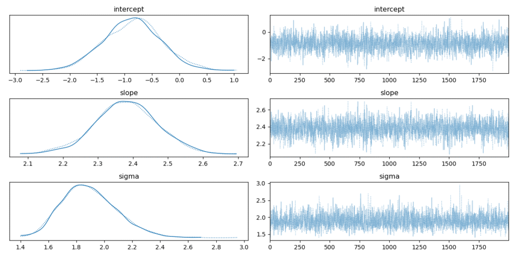
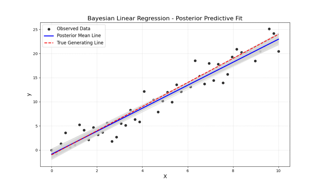
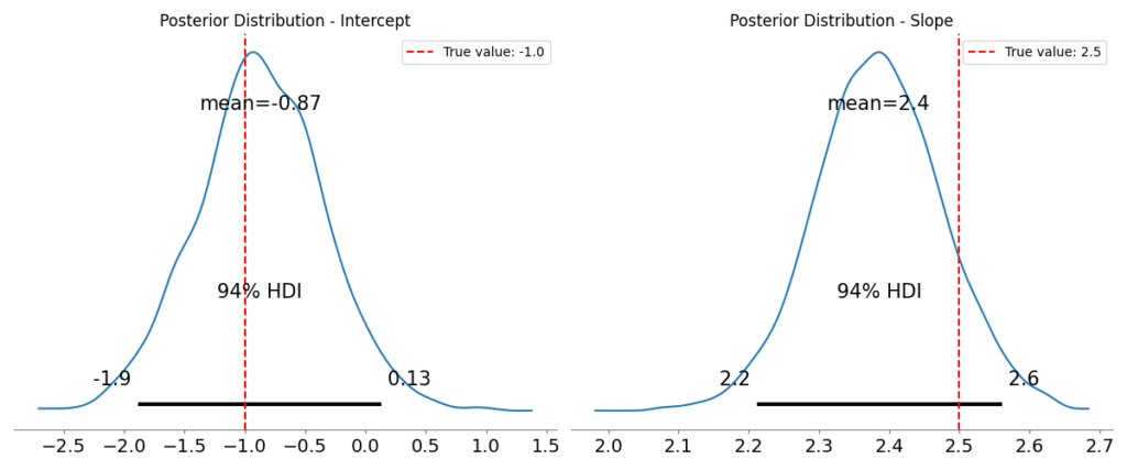
The output of this code is profoundly insightful. The trace plot shows the posterior distributions for the intercept and slope. They are not single values but distributions, indicating our uncertainty about their true values. The second plot visualizes this uncertainty directly on the data. The cloud of gray lines represents different possible regression lines sampled from our posterior. This immediately communicates the model’s confidence: where the lines are tightly packed, the model is certain; where they spread out, it is uncertain.
Computational Exercises
- Sequential Updates: Modify the coin-flipping example to perform the Bayesian update sequentially. Start with the \(\text{Beta}(1, 1)\) prior. Process one data point at a time, using the posterior from the previous step as the prior for the next. Plot the evolution of the posterior distribution after 1, 5, 10, and 20 flips. What do you observe about how the posterior changes as more data is incorporated?
- Prior Sensitivity Analysis: Rerun the Bayesian linear regression model with three different sets of priors for the slope and intercept:a. Weakly Informative (as above): pm.Normal(‘slope’, mu=0, sigma=10)b. Highly Informative (but wrong): pm.Normal(‘slope’, mu=10, sigma=1)c. Very Uninformative: pm.Normal(‘slope’, mu=0, sigma=100)Compare the posterior distributions and the summary statistics for each. How does the choice of prior affect the result when the dataset is small (e.g., n=50)? What would you expect to happen if you had a very large dataset (e.g., n=5000)?
Real-World Problem Applications
The power of Bayesian methods extends across all domains of AI.
- Natural Language Processing (NLP): Latent Dirichlet Allocation (LDA) is a classic Bayesian model used for topic modeling. It treats documents as a mixture of topics and topics as a distribution of words, using Bayesian inference to uncover the hidden thematic structure in a large corpus of text.
- Computer Vision: Bayesian methods are used in object tracking algorithms (like the Kalman filter, a special case of a Bayesian model) to maintain a belief state about an object’s position and velocity, updating this belief with each new video frame.
- Reinforcement Learning: Bayesian approaches can be used to model uncertainty in the environment’s dynamics or rewards, leading to more exploration-efficient agents that can balance exploiting known good actions with exploring uncertain ones.
- A/B Testing: Instead of waiting for a classical significance test to complete, Bayesian A/B testing can provide the probability that variant A is better than variant B at any point in time, allowing for more flexible business decisions.
Industry Applications and Case Studies
The theoretical elegance of Bayesian methods translates into significant business value and robust solutions across various industries. Their ability to quantify uncertainty and incorporate prior knowledge makes them uniquely suited for high-stakes decision-making.
- Pharmaceuticals and Clinical Trials: Drug development is a lengthy and expensive process. Bayesian methods are increasingly used to design more efficient clinical trials. Adaptive trials can be designed where the parameters of the trial (e.g., dosage, number of participants in each arm) are modified as data is collected. If one treatment is clearly showing superior results early on, more patients can be allocated to that arm. This allows for smaller, faster, and more ethical trials. For example, the I-SPY 2 trial for breast cancer uses a Bayesian adaptive design to screen multiple experimental drugs simultaneously, graduating effective ones to larger trials more quickly. The business impact is a reduction in R&D costs and a faster time-to-market for life-saving drugs.
- Finance and Algorithmic Trading: Financial markets are inherently noisy and non-stationary. A trading algorithm needs to know when its model is uncertain. Bayesian models, such as Gaussian Processes for time-series forecasting, can predict not just the future price of an asset but also a credible interval around that prediction. When the interval is wide, it signals high volatility or model uncertainty, and the algorithm can reduce its position size or refrain from trading. This prevents large losses during unpredictable market conditions. The technical challenge is the high-frequency nature of the data, requiring fast inference methods like VI or specialized hardware. The ROI comes from improved risk management and capital preservation.
- Supply Chain and Inventory Management: Companies like Amazon and Walmart need to predict demand for millions of items at thousands of locations. A point estimate for demand is insufficient; they need to understand the full distribution of possible demand to optimize inventory. A Bayesian hierarchical model can be used to solve this. It can model demand for each product at each location, while sharing statistical strength across similar products, locations, or time periods (e.g., learning a general “seasonality” effect). This allows for accurate demand forecasting even for items with sparse sales data. The output is a posterior distribution for demand, which can be used to calculate the optimal stock level to meet a target service level (e.g., 99% probability of not stocking out), directly minimizing both holding costs and lost sales.
Best Practices and Common Pitfalls
While powerful, the Bayesian workflow requires care and expertise. Adhering to best practices is crucial for building models that are not only statistically sound but also reliable and maintainable in a professional setting.
- Start Simple and Iterate: The temptation to build a complex, all-encompassing hierarchical model from the start is a common pitfall. This often leads to models that are difficult to debug and take forever to run. The best practice is to start with the simplest possible model that captures the core of your problem. Use posterior predictive checks to diagnose misfit, and only add complexity (e.g., hierarchical structures, interaction terms) when the data and diagnostics justify it.
- Think Carefully About Priors (Prior Predictive Checks): Priors are a feature, not a bug. However, a poorly chosen prior can unintentionally constrain your model or lead to nonsensical results. A common mistake is to use “uninformative” priors without checking their implications. A
Uniform(0, 1e9)prior on a standard deviation parameter might seem uninformative, but it can induce strange behavior. The best practice is to perform prior predictive checks: generate data from your model using only your priors (i.e., before you’ve seen the data). If the generated data looks nothing like the plausible real-world data, your priors are likely problematic. - Diagnose Your Chains (MCMC Convergence): When using MCMC, it’s not enough to just run the sampler and take the results. You must verify that the algorithm has converged to the target posterior distribution. A common pitfall is to run too few samples or have chains that get stuck in a local mode. Best practices include: inspecting trace plots for “fuzzy caterpillar” behavior (good mixing), checking that the \(\hat{R}\) (R-hat) statistic is close to 1.0 (indicating convergence across chains), and ensuring the effective sample size (ESS) is sufficiently high for stable estimates.
- Embrace the Full Posterior: A frequent mistake is to run a full Bayesian analysis and then only report a single point estimate (like the posterior mean). This discards the richest part of the output: the uncertainty quantification. Best practices involve visualizing the full posterior distributions, reporting credible intervals, and using the full posterior predictive distribution to propagate uncertainty into your final predictions and decisions.
Warning: MCMC algorithms can be sensitive to the parameterization of the model. If you are getting convergence warnings (like divergences in HMC/NUTS), it often indicates a problem with the model’s geometry. Reparameterizing the model (e.g., using a non-centered parameterization in a hierarchical model) can often resolve these issues and lead to much more efficient sampling.
Hands-on Exercises
These exercises are designed to reinforce the chapter’s concepts, progressing from foundational understanding to practical application.
- The German Tank Problem: During WWII, the Allies used Bayesian inference to estimate the total number of tanks Germany was producing. Assume Germany numbers its tanks sequentially from 1 to \(N\). The Allies capture a small number of tanks and observe their serial numbers.
- Objective: Estimate the total number of tanks, \(N\).
- Task: You have captured 5 tanks with serial numbers: 16, 23, 45, 60, 98. Assume a discrete uniform prior for \(N\) from 1 to 500 (i.e., \(P(N) = 1/500\) for \(N \in [1, 500]\)). The likelihood of observing the data given \(N\) is \(1/N^k\) if \(N \ge \max(\text{data})\) and 0 otherwise, where \(k\) is the number of captured tanks.
- Implementation: Write a Python script to calculate the unnormalized posterior probability for each possible value of \(N\). Plot the posterior distribution for \(N\). What is the most probable value for \(N\) (the posterior mode)?
- Bayesian Logistic Regression for Classification: Using the
scikit-learnbreast cancer dataset, build a Bayesian logistic regression model using PyMC to predict whether a tumor is malignant or benign based on a single feature (e.g., ‘mean radius’).- Objective: Implement a probabilistic classifier and interpret its output.
- Task:
- Load the data and select one feature.
- Define a logistic regression model in PyMC. You will need priors for the intercept and the slope.
- The likelihood will be a Bernoulli distribution, with the probability parameter \(p\) being the output of the logistic (sigmoid) function: \(p = \text{sigmoid}(\alpha + \beta x)\).
- Run the MCMC sampler.
- Plot the posterior distributions for the slope and intercept. Is there strong evidence that ‘mean radius’ is associated with malignancy (i.e., is the 95% credible interval for the slope far from zero)?
- Plot the predicted probability of malignancy as a function of ‘mean radius’, including the uncertainty (credible interval) around the prediction curve.
- Team Project – Hierarchical Modeling: Imagine you are analyzing student test scores from several different schools. A simple approach would be to model each school independently or to pool all the data and ignore the school structure. A better, Bayesian approach is to use a hierarchical model.
- Objective: Design and justify a hierarchical model for analyzing test scores.
- Task (as a team):
- Simulate data: Create a synthetic dataset of test scores for 5 different schools. Make the average score in each school different, but have them all drawn from a common “national average” distribution.
- Model Design: Whiteboard the model architecture. You’ll have a parameter for each school’s average score. Instead of giving these independent priors, the hierarchical model assumes that each school’s average is drawn from a higher-level distribution (the hyper-prior), which represents the national average and variation.
- Implementation (Optional): If time permits, try to implement this model in PyMC.
- Discussion: What are the advantages of this approach compared to modeling each school separately or pooling all the data? How does this model perform “shrinkage,” pulling the estimates for schools with little data towards the overall average?
Tools and Technologies
A modern AI engineer’s toolkit for Bayesian modeling is rich and powerful, built primarily on the Python ecosystem.
- PyMC: A flexible and powerful probabilistic programming library in Python. It uses Theano (or JAX in newer versions) as its computational backend and features state-of-the-art samplers like NUTS. Its intuitive syntax makes it excellent for defining custom Bayesian models.
- Stan: A standalone platform and probabilistic programming language implemented in C++. It is renowned for its robust and highly optimized HMC sampler. It has interfaces for most major data science languages, including Python (via
CmdStanPyor the olderPyStan). It is often favored in academia for its statistical rigor. - Pyro and NumPyro: Probabilistic programming languages developed by Uber AI. Pyro is built on PyTorch, and NumPyro is built on JAX. They are particularly well-suited for deep generative models and scalable Variational Inference, making them a top choice for Bayesian deep learning research.
- ArviZ: A crucial library for the exploratory analysis of Bayesian models. It works seamlessly with PyMC, Stan, NumPyro, and others to provide functions for visualizing posterior distributions, creating trace plots, calculating summary statistics (like \(\hat{R}\) and ESS), and performing posterior predictive checks.
- Scikit-learn: While primarily a Frequentist library, it contains some Bayesian implementations, such as
BayesianRidgeregression andGaussianNB(Naive Bayes) classifier, which can be useful for simpler applications or as baselines.
| PPL | Primary Language/Backend | Key Strengths | Best For |
|---|---|---|---|
| PyMC | Python / PyTensor (formerly Theano/JAX) | Flexible, intuitive Python syntax. Great for custom models. Excellent integration with ArviZ for diagnostics. Strong community. | General-purpose Bayesian modeling, from simple regressions to complex hierarchical models. A great starting point for practitioners. |
| Stan | Stan (own language) / C++ | Extremely fast and robust NUTS sampler. Considered the gold standard for MCMC performance and statistical rigor. | Statisticians and researchers who need maximum MCMC efficiency and reliability. When performance is critical. |
| Pyro / NumPyro | Python / PyTorch (Pyro) or JAX (NumPyro) | Designed for deep generative models and scalable Variational Inference. Leverages GPU acceleration from its backends. | Bayesian Deep Learning, large-scale VI, and research in modern probabilistic models. |
Note: When setting up your environment, it’s best to use a package manager like
condaorpipwithin a virtual environment. For example:pip install pymc arviz numpy matplotlib scikit-learn. This ensures that you have compatible versions of all necessary libraries.
Summary
This chapter provided a comprehensive introduction to the Bayesian paradigm for machine learning, emphasizing its role in managing uncertainty.
- Core Idea: Bayesian inference updates our beliefs (prior) in light of new data (likelihood) to form an updated belief (posterior). Probability is treated as a degree of belief, not a long-run frequency.
- Bayes’ Theorem: The mathematical engine of this process is \( P(\theta | D) \propto P(D | \theta) P(\theta) \).
- Uncertainty Quantification: The output of a Bayesian analysis is not a single point estimate but a full posterior distribution, which naturally provides measures of uncertainty like credible intervals.
- Practical Implementation: Modern Probabilistic Programming Languages (PPLs) like PyMC and Stan make it feasible to define and solve complex Bayesian models using powerful inference algorithms like NUTS (MCMC) and VI.
- AI Engineering Advantage: By embracing uncertainty, we can build more robust, reliable, and interpretable AI systems, from safer autonomous vehicles to more efficient business operations. The skills gained in this chapter are directly applicable to a wide range of advanced AI domains.
Further Reading and Resources
- Gelman, A., Carlin, J. B., Stern, H. S., Dunson, D. B., Vehtari, A., & Rubin, D. B. (2013). Bayesian Data Analysis, Third Edition. CRC Press. (The definitive graduate-level textbook on the subject, often called “the BDA”).
- McElreath, R. (2020). Statistical Rethinking: A Bayesian Course with Examples in R and Stan, Second Edition. CRC Press. (An exceptionally intuitive and example-driven introduction to Bayesian modeling).
- The PyMC Documentation and Examples: (Official website:
pymc.io) An excellent resource with numerous tutorials and case studies for practical implementation. - Kruschke, J. K. (2014). Doing Bayesian Data Analysis, Second Edition: A Tutorial with R, JAGS, and Stan. Academic Press. (A very accessible, ground-up introduction with great explanations).
- Stan User’s Guide and Reference Manual: (Official website:
mc-stan.org) The official documentation for the Stan language, providing deep insights into the underlying algorithms and best practices. - Bishop, C. M. (2006). Pattern Recognition and Machine Learning. Springer. (Chapter 2 provides a concise and clear introduction to probability theory from both Bayesian and Frequentist perspectives).
- ArviZ Documentation: (Official website:
https://python.arviz.org/en/0.14.0/index.html) Essential reading for learning how to properly diagnose and visualize the output of your Bayesian models.
Glossary of Terms
- Bayes’ Theorem: The fundamental formula for Bayesian inference that relates the conditional and marginal probabilities of two random events.
- Posterior Distribution: The probability distribution of a parameter after observing the data; it represents our updated belief.
- Prior Distribution: The probability distribution of a parameter before observing the data; it represents our initial belief.
- Likelihood: The probability of observing the data given a specific value of the parameter. It is the function that connects the data to the model parameters.
- Evidence (Marginal Likelihood): The total probability of the data, calculated by integrating the likelihood over the prior. It acts as a normalization constant.
- Credible Interval: The Bayesian analogue of a confidence interval. A 95% credible interval for a parameter is a range within which the parameter lies with 95% probability, according to the posterior distribution.
- Conjugate Prior: A prior distribution that, when combined with a given likelihood, results in a posterior distribution from the same probability distribution family.
- MCMC (Markov Chain Monte Carlo): A class of algorithms for sampling from a probability distribution. It is the primary computational tool for approximating complex posterior distributions.
- NUTS (No-U-Turn Sampler): An advanced and efficient MCMC algorithm, a variant of Hamiltonian Monte Carlo, used by default in PyMC and Stan.
- VI (Variational Inference): An alternative to MCMC that frames inference as an optimization problem. It is often faster but provides an approximation to the true posterior.
- PPL (Probabilistic Programming Language): A high-level language (like PyMC or Stan) that allows users to define probabilistic models and automatically run inference.
