
Chapter 8: Basic Matrix Operations and Properties
Chapter Objectives
Upon completing this chapter, you will be able to:
- Understand the fundamental definition of a matrix and its role as a core data structure in machine learning and computational mathematics.
- Implement fundamental matrix operations—including addition, scalar multiplication, matrix-vector multiplication, and matrix-matrix multiplication—using Python and the NumPy library.
- Analyze the mathematical properties of matrix operations, such as associativity and distributivity, and identify common pitfalls like the non-commutativity of matrix multiplication.
- Apply matrix operations to represent and solve practical problems, such as performing linear transformations on data and setting up the foundational calculations for neural network layers.
- Optimize computational code by leveraging vectorized matrix operations to avoid inefficient loops and enhance performance.
- Design simple computational workflows that use matrices to represent datasets and model parameters, forming the building blocks for more complex AI systems.
Introduction
In the landscape of modern artificial intelligence, from the intricate layers of a deep neural network to the elegant logic of a support vector machine, a single mathematical construct reigns supreme: the matrix. At its essence, a matrix is a rectangular array of numbers, symbols, or expressions, arranged in rows and columns. Yet, this simple structure is the bedrock upon which the vast edifice of computational intelligence is built. It is the language through which we describe data, define transformations, and encode the parameters that models learn from experience.
This chapter introduces the fundamental operations and properties of matrices, a topic that is not merely a prerequisite for AI engineering but its computational heart. We will explore how these collections of numbers are manipulated through operations like addition, multiplication, and transposition. These are not abstract mathematical exercises; they are the very calculations that power image recognition, natural language processing, and predictive analytics. For instance, when a neural network “learns,” it is iteratively adjusting the values within its weight matrices. When an image is rotated or scaled by a computer graphics program, a matrix multiplication is performing the transformation.
We will move from the theoretical underpinnings of these operations to their practical implementation. You will learn to harness the power of Python’s NumPy library, the industry-standard tool for numerical computation, to perform these operations with unparalleled efficiency. By mastering the concepts in this chapter, you will gain the foundational skills necessary to understand, build, and optimize the complex algorithms that drive the AI revolution. This is the starting point for demystifying what happens inside the “black box” of machine learning and beginning your journey as a proficient and insightful AI engineer.
Technical Background
The journey into machine learning is paved with linear algebra. While the field is vast, a solid understanding of its fundamental unit of computation—the matrix—is non-negotiable. Matrices provide a powerful and efficient formalism for organizing data and expressing complex mathematical operations, making them indispensable in AI. This section lays the theoretical groundwork for matrix operations, exploring not just how to perform them, but why they behave the way they do and what that means for their application in machine learning.
Fundamental Concepts and Definitions
Core Terminology and Mathematical Foundations
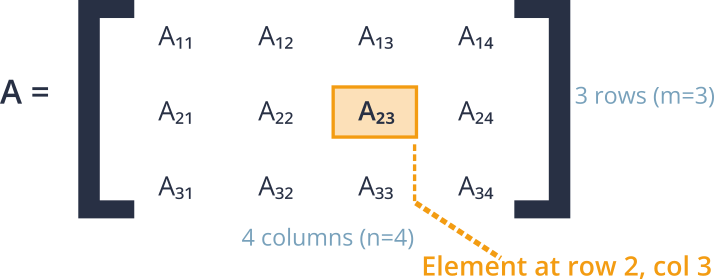
A matrix is a rectangular grid of numbers arranged into rows and columns. We describe the size, or dimension, of a matrix by the number of rows and columns it contains. A matrix with \(m\) rows and \(n\) columns is called an \(m \times n\) matrix (read “m by n”). Each element within the matrix is identified by its position, typically using a subscript notation like \(A_{ij}\), which denotes the element in the \(i\)-th row and \(j\)-th column of matrix A.
A vector is a special case of a matrix, having only one column (a column vector) or one row (a row vector). Vectors are the primary way we represent individual data points in machine learning. For example, a user’s profile with features like age, income, and hours spent online could be represented as a vector [34, 65000, 15]. A collection of these vectors, representing multiple users, naturally forms a matrix where each row corresponds to a user. A single number is called a scalar, which can be thought of as a \(1 \times 1\) matrix.
The power of this structure lies in its ability to organize related data. For a dataset of house prices, one matrix could hold all the feature data (square footage, number of bedrooms, location), with each row representing a different house and each column a different feature. Another vector could hold the corresponding sale prices. The goal of a linear regression model, then, is to find a set of weights—another vector—that can be multiplied by the feature matrix to approximate the price vector. This elegant representation turns a complex statistical problem into a structured set of matrix operations.
Special Types of Matrices
In our work, we will frequently encounter several special types of matrices. The most common are square matrices, where the number of rows equals the number of columns (\(m = n\)). Within this category, a few are particularly important.
The identity matrix, denoted as I, is a square matrix with ones on its main diagonal (from the top-left to the bottom-right) and zeros everywhere else. The identity matrix is the matrix equivalent of the number 1; multiplying any matrix A by I (of an appropriate size) leaves A unchanged. This property, \(A \cdot I = I \cdot A = A\), is crucial for solving systems of linear equations and for deriving many machine learning algorithms.
The zero matrix is a matrix of any dimension filled entirely with zeros. It is the additive identity, meaning that adding it to any matrix A results in A.
A diagonal matrix is a square matrix where all off-diagonal elements are zero. The identity matrix is a specific type of diagonal matrix. Diagonal matrices are computationally efficient to work with, especially for inversion and multiplication, and they appear in various optimization algorithms and data transformation techniques like Principal Component Analysis (PCA).
Commonly Encountered Special Matrices
| Matrix Type | Definition | Example (3×3) | Key Property |
|---|---|---|---|
| Square Matrix | A matrix with an equal number of rows and columns (m = n). | Any 3×3 matrix. | Required for concepts like determinants, eigenvalues, and identity matrices. |
| Identity Matrix (I) | A square matrix with 1s on the main diagonal and 0s elsewhere. | [[1, 0, 0], [0, 1, 0], [0, 0, 1]] |
Multiplicative identity: A @ I = A. |
| Zero Matrix | A matrix of any dimension where all elements are zero. | [[0, 0, 0], [0, 0, 0], [0, 0, 0]] |
Additive identity: A + 0 = A. |
| Diagonal Matrix | A square matrix where all off-diagonal elements are zero. | [[3, 0, 0], [0, -5, 0], [0, 0, 2]] |
Computationally efficient for multiplication and inversion. |
| Symmetric Matrix | A square matrix that is equal to its own transpose (A = AT). | [[1, 7, 3], [7, 4, -5], [3, -5, 6]] |
Common in statistics (e.g., covariance matrices); has real eigenvalues. |
Finally, the transpose of a matrix A, denoted as \(A^T\), is a new matrix formed by swapping its rows and columns. The element at position \((i, j)\) in A becomes the element at position \((j, i)\) in \(A^T\). If A is an \(m \times n\) matrix, then \(A^T\) will be an \(n \times m\) matrix. Transposition is a fundamental operation used extensively in machine learning, for example, to align the dimensions of vectors and matrices for multiplication in the weight update step of a neural network.
Core Matrix Operations
Matrix Addition and Scalar Multiplication
The simplest matrix operations are element-wise. Matrix addition is defined for two matrices of the same dimensions. To add two matrices, A and B, we simply add their corresponding elements. If \(C = A + B\), then each element of C is given by \(C_{ij} = A_{ij} + B_{ij}\). This operation is both commutative (\(A + B = B + A\)) and associative (\(A + (B + C) = (A + B) + C\)), properties that make it behave intuitively like the addition of scalars. In machine learning, this operation is often used to add a bias term to a layer’s output. For example, if a matrix represents the outputs of several neurons for a batch of data, a bias vector can be added to this matrix to shift the activation function.

Scalar multiplication involves multiplying every element of a matrix by a single number (a scalar). If \(c\) is a scalar and A is a matrix, the product \(c \cdot A\) is a matrix where each element is \(c \cdot A_{ij}\). This operation is used to scale data or to control the learning rate in optimization algorithms. For example, in gradient descent, the calculated gradient (a matrix or vector) is multiplied by a small scalar learning rate before being subtracted from the model’s weight matrix. This scaling ensures that the weight updates are small, preventing the optimization process from overshooting the minimum.
These two operations—addition and scalar multiplication—form the basis of what is known as a vector space. The fact that matrices (of the same size) obey these properties allows us to treat them as vectors in a higher-dimensional space, a conceptual leap that underpins much of the geometric interpretation of machine learning.
Matrix Multiplication: The Engine of Transformation
Matrix multiplication is arguably the most important operation in all of linear algebra for AI applications. Unlike addition, it is not performed element-wise, and its mechanics are more complex but far more powerful. The product of two matrices, A and B, is defined only if the number of columns in A is equal to the number of rows in B. If A is an \(m \times n\) matrix and B is an \(n \times p\) matrix, their product, \(C = AB\), will be an \(m \times p\) matrix.
Each element \(C_{ij}\) of the resulting matrix is calculated by taking the dot product of the \(i\)-th row of A and the \(j\)-th column of B. The dot product is the sum of the products of their corresponding elements.
Mathematically,
$$[C_{ij} = \sum_{k=1}^{n} A_{ik} \cdot B_{kj}]$$
graph TD
    subgraph Legend
        direction LR
        L1(Data / Input):::dataStyle
        L2(Process):::processStyle
        L3(Result):::successStyle
    end

    subgraph "Calculating Element C_ij in Product Matrix C = A @ B"
        A[("<b>Matrix A</b><br><i>m x n</i>")]:::dataStyle
        B[("<b>Matrix B</b><br><i>n x p</i>")]:::dataStyle

        A --> R{{"Extract Row <i>i</i> from A<br>(Size: 1 x n)"}}:::processStyle
        B --> C{{"Extract Column <i>j</i> from B<br>(Size: n x 1)"}}:::processStyle

        R --> DP["Perform Dot Product<br>C_ij = Σ (A_ik * B_kj)<br>for k=1 to n"]:::processStyle
        C --> DP

        DP --> E{"(Element C_ij<br><i>A single scalar value</i>)"}:::successStyle
        E --> F[("<b>Result Matrix C</b><br><i>m x p</i>")]:::successStyle

        subgraph "Repeat for all i, j"
           direction LR
           E
        end

    end

    classDef dataStyle fill:#9b59b6,stroke:#9b59b6,stroke-width:2px,color:#ebf5ee
    classDef processStyle fill:#78a1bb,stroke:#78a1bb,stroke-width:1px,color:#283044
    classDef successStyle fill:#2d7a3d,stroke:#2d7a3d,stroke-width:2px,color:#ebf5ee
This operation is the workhorse of neural networks. If we have a matrix of input data (where each row is a data sample) and a weight matrix for a neural network layer (where each column represents a neuron’s weights), their product gives the pre-activation outputs for each neuron for each data sample. It is a compact and incredibly efficient way to perform a massive number of calculations simultaneously.
A critical property of matrix multiplication is that it is not commutative; that is, in general, \(AB \neq BA\). The order of multiplication matters immensely. Multiplying a data matrix by a weight matrix is a valid operation that transforms data, but reversing the order may not even be dimensionally possible, and if it is, it will produce a result with a completely different meaning. However, matrix multiplication is associative (\(A(BC) = (AB)C\)) and distributive over addition (\(A(B+C) = AB + AC\)). These properties are heavily relied upon in algebraic manipulations of machine learning formulas and in optimizing the computational graphs used by deep learning frameworks.
The Transpose and Its Properties
The transpose operation, while simple, has profound implications. As previously defined, the transpose \(A^T\) of a matrix A is found by flipping the matrix over its main diagonal. This operation has several useful properties:
- \((A^T)^T = A\): Transposing a matrix twice returns the original matrix.
- \((A+B)^T = A^T + B^T\): The transpose of a sum is the sum of the transposes.
- \((cA)^T = cA^T\): A scalar can be factored out of a transpose operation.
- \((AB)^T = B^T A^T\): The transpose of a product is the product of the transposes in reverse order. This last property is particularly important and frequently used in deriving machine learning update rules, especially in the context of backpropagation.
A special and highly useful type of matrix is a symmetric matrix, which is a square matrix that is equal to its own transpose (\(A = A^T\)). Covariance matrices, which are fundamental in many statistical and machine learning methods like PCA, are always symmetric. This symmetry has important implications for their properties, such as guaranteeing that their eigenvalues are real.
In practice, the transpose is often a utility for aligning dimensions. For example, to calculate the dot product of two column vectors u and v, we can’t multiply them directly as \((n \times 1)\) by \((n \times 1)\) matrices. Instead, we compute it as \(u^T v\), which is a \((1 \times n)\) matrix (a row vector) multiplied by an \((n \times 1)\) matrix (a column vector), resulting in a \(1 \times 1\) matrix—a scalar, which is the dot product. This technique is ubiquitous in AI literature and code.
Practical Examples and Implementation
Theory provides the “what” and “why,” but practical implementation provides the “how.” In modern AI engineering, matrix operations are rarely performed by hand. Instead, we leverage highly optimized numerical computing libraries. The undisputed leader in the Python ecosystem is NumPy (Numerical Python), which provides a powerful ndarray object for representing matrices and a comprehensive library of functions for manipulating them with C-like speed.
Mathematical Concept Implementation with NumPy
Let’s translate the core matrix operations into working Python code. The foundation of NumPy is the ndarray, which we will use to create vectors (1D arrays) and matrices (2D arrays).
Note: By convention, we import NumPy with the alias
np. All the following examples assumeimport numpy as nphas been executed.
First, let’s define a few matrices and vectors to work with.
# A 3x3 matrix
A = np.array([
    [1, 2, 3],
    [4, 5, 6],
    [7, 8, 9]
])

# Another 3x3 matrix
B = np.array([
    [9, 8, 7],
    [6, 5, 4],
    [3, 2, 1]
])

# A 3x1 column vector
v = np.array([[10], [20], [30]])

# A scalar
c = 2
Matrix Addition and Scalar Multiplication
These operations are straightforward and intuitive in NumPy. Standard arithmetic operators (+, -, *, /) work element-wise.
# Matrix Addition
C = A + B
print("A + B:\n", C)

# Scalar Multiplication
D = c * A
print("\n2 * A:\n", D)
This demonstrates the power of vectorization. NumPy performs these operations in highly optimized, pre-compiled C code, avoiding slow, explicit for loops in Python. A manual implementation would require nested loops, which is significantly less efficient.
Tip: Always use NumPy’s vectorized operations instead of writing your own loops for matrix arithmetic. The performance difference can be several orders of magnitude, especially for large matrices.
Matrix Transpose
Transposing a matrix in NumPy is trivial. Every ndarray has a .T attribute that returns the transposed matrix.
# Transposing matrix A
A_t = A.T
print("Transpose of A:\n", A_t)

# Transposing vector v (turns a column vector into a row vector)
v_t = v.T
print("\nTranspose of v:\n", v_t)
print("Shape of v:", v.shape) # (3, 1)
print("Shape of v_t:", v_t.shape) # (1, 3)
AI/ML Application Examples
Matrix-Vector Multiplication: Applying Weights to a Single Data Point
In machine learning, a fundamental operation is applying a set of learned weights to an input data sample. Let’s say we have a single data point represented by a vector x with 3 features, and a simple linear model has learned a set of weights, represented by a matrix W.
# A single data point with 3 features (as a 1x3 row vector)
x = np.array([[1.5, 2.0, 0.5]]) # e.g., sq_ft, num_bedrooms, age_of_house

# A weight matrix for a layer with 2 output neurons.
# Dimensions: 3 features (rows) x 2 neurons (columns)
W = np.array([
    [0.1, 0.5],  # Weights for feature 1 connecting to neuron 1 and 2
    [0.2, 0.8],  # Weights for feature 2 connecting to neuron 1 and 2
    [0.3, -0.4]  # Weights for feature 3 connecting to neuron 1 and 2
])

# To multiply, the dimensions must align: (1x3) @ (3x2)
# The @ operator is used for matrix multiplication in Python 3.5+
output = x @ W
print("Input shape:", x.shape)
print("Weight shape:", W.shape)
print("Output shape:", output.shape)
print("Output of the layer:", output) # Result is a 1x2 vector
The result, [[0.7, 1.95]], represents the output values of the two neurons for the input x. This single operation is a building block of a neural network’s forward pass.
Matrix-Matrix Multiplication: Processing a Batch of Data
AI models are almost always trained on batches of data for efficiency. We can represent a batch of data as a matrix where each row is a data point. Matrix-matrix multiplication allows us to process the entire batch in one go.
# A batch of 4 data points, each with 3 features
X_batch = np.array([
    [1.5, 2.0, 0.5],
    [2.5, 3.0, 1.0],
    [0.5, 1.0, 0.2],
    [1.8, 2.2, 0.8]
])

# Use the same weight matrix W
# Dimensions: (4x3) @ (3x2) -> (4x2)
batch_output = X_batch @ W

print("Batch input shape:", X_batch.shape)
print("Weight shape:", W.shape)
print("Batch output shape:", batch_output.shape)
print("\nOutput for the entire batch:\n", batch_output)
The resulting \(4 \times 2\) matrix contains the outputs for each of the 4 data points. This is computationally far more efficient than iterating through each data point and performing a matrix-vector multiplication.
Visualization and Interactive Examples
Matrices can be interpreted as linear transformations that stretch, shrink, rotate, or skew space. Visualizing this can provide a much deeper intuition for what matrix multiplication actually does. We can use Matplotlib to plot vectors and see how they change after being multiplied by a matrix.
Let’s define a 2D vector and a transformation matrix.
import matplotlib.pyplot as plt
import numpy as np

# Original vector
p = np.array([1, 2])

# Transformation matrix (this one rotates and scales)
T = np.array([
    [0.5, -1],
    [1, 0.5]
])

# Apply the transformation
p_transformed = p @ T

# Plotting
plt.figure(figsize=(6, 6))
# Plot original vector
plt.quiver(0, 0, p[0], p[1], angles='xy', scale_units='xy', scale=1, color='blue', label='Original Vector')
# Plot transformed vector
plt.quiver(0, 0, p_transformed[0], p_transformed[1], angles='xy', scale_units='xy', scale=1, color='red', label='Transformed Vector')

plt.xlim(-3, 3)
plt.ylim(-3, 3)
plt.axhline(0, color='grey', lw=0.5)
plt.axvline(0, color='grey', lw=0.5)
plt.grid(True)
plt.legend()
plt.title("Linear Transformation of a Vector")
plt.show()
This visualization clearly shows that matrix multiplication is not just an abstract calculation; it’s a geometric operation. This is fundamental to computer graphics and also to understanding how neural networks manipulate data representations in high-dimensional spaces.
Computational Exercises
- Manual vs. NumPy: Given matrices \(A = \begin{pmatrix} 2 & 1 \ 0 & 3 \end{pmatrix}\) and \(B = \begin{pmatrix} -1 & 2 \ 4 & -1 \end{pmatrix}\), calculate the product \(AB\) first by hand. Then, verify your result using NumPy. Manual Calculation:
\[C_{11} = (2 \cdot -1) + (1 \cdot 4) = 2\]
\[C_{12} = (2 \cdot 2) + (1 \cdot -1) = 3\]
\[C_{21} = (0 \cdot -1) + (3 \cdot 4) = 12\]
\[C_{22} = (0 \cdot 2) + (3 \cdot -1) = -3\]
So, \(AB = \begin{pmatrix} 2 & 3 \ 12 & -3 \end{pmatrix}\). NumPy Verification:A = np.array([[2, 1], [0, 3]]) B = np.array([[-1, 2], [4, -1]]) C = A @ B print("A @ B:\n", C) - Dimensionality Errors: In NumPy, try to compute
A + vandA @ vwhereAis \(3 \times 3\) andvis \(3 \times 1\). What happens? Why? Now, try to computeA @ v.T. Does it work? Why or why not? This exercise highlights the strict dimensional requirements of matrix operations. Warning: Mismatched dimensions are one of the most common sources of bugs in machine learning code. Always be mindful of the shapes of your matrices.print(matrix.shape)is your best debugging friend.
Industry Applications and Case Studies
The abstract power of matrix operations translates into tangible value across countless industries. They are not just academic curiosities; they are the engines of modern data-driven products and services.
- Computer Vision (Image Manipulation): Every digital image is fundamentally a matrix (or three matrices for RGB colors), where each element represents a pixel’s intensity. Matrix operations are used for filtering, resizing, rotation, and feature detection. For example, applying a convolution—a core operation in Convolutional Neural Networks (CNNs)—involves sliding a small weight matrix (a kernel) over the image matrix and performing element-wise multiplication and summation. Companies like Google Photos and Adobe use these techniques for everything from sharpening images to identifying faces and objects within them. The business value lies in automated photo organization, enhanced user experience, and powerful creative tools.
- Natural Language Processing (NLP) and Recommender Systems: In NLP, words and sentences are converted into numerical vectors (embeddings). A matrix can represent a collection of these embeddings. Recommender systems, like those at Netflix and Amazon, use a technique called matrix factorization. They start with a massive, sparse matrix of user-item interactions (e.g., user ratings for movies). The goal is to approximate this large matrix as the product of two smaller, dense matrices: a “user-feature” matrix and an “item-feature” matrix. Multiplying these two matrices back together fills in the missing values of the original, providing predictions for what a user might like. This directly drives user engagement and sales by personalizing content.
- Simulation and Scientific Computing: In fields from aerospace engineering to financial modeling, systems of linear equations are used to model complex, real-world phenomena. These systems are represented in the form \(Ax = b\), where A is a matrix of coefficients, x is a vector of unknown variables, and b is a vector of outcomes. Solving for x requires matrix operations, specifically finding the inverse of A. Companies like Boeing use these methods to simulate airflow over a wing, while hedge funds at Renaissance Technologies use them to model market dynamics, enabling them to make predictions worth billions. The ROI is immense, stemming from optimized designs, risk reduction, and predictive accuracy.
Best Practices and Common Pitfalls
While powerful, matrix operations must be handled with care. Writing efficient, scalable, and correct AI code requires adhering to best practices and being aware of common errors.
- Embrace Vectorization, Avoid Loops: As emphasized earlier, the single most important performance practice is to use the vectorized operations provided by libraries like NumPy and TensorFlow/PyTorch. A
forloop in Python that iterates over matrix elements can be 100x to 1000x slower than the equivalent vectorized operation. This is because the libraries execute these operations in low-level, compiled code (C, C++, or CUDA for GPUs) that can process data in parallel chunks. - The Curse (and Blessing) of Dimensionality: The most frequent bug in ML programming is the
DimensionMismatchError. This happens when you try to add or multiply matrices with incompatible shapes. The best practice is to be obsessive about tracking matrix dimensions. Useprint(my_matrix.shape)liberally during development. Before writing a line of code for an operation, mentally (or on paper) check the dimensions: “I’m multiplying a \((512 \times 784)\) matrix with a \((784 \times 128)\) matrix. The result should be \((512 \times 128)\).” This simple habit prevents countless hours of debugging. - Numerical Stability: When working with very large or very small numbers, standard floating-point arithmetic can lead to issues like overflow (numbers becoming infinitely large) or underflow (numbers becoming zero). This can derail model training. Best practices include data normalization (scaling input features to a small range, like 0 to 1) and using numerically stable functions provided by libraries (e.g.,
log-sum-exptrick for softmax calculations) instead of implementing them naively. - Memory Management: Matrices, especially in deep learning, can be enormous. A single matrix of \(10,000 \times 10,000\) 32-bit floats consumes 400 MB of memory. Be mindful of how many large matrices you are holding in memory at once. Use data types with lower precision (e.g.,
float16) if possible, and leverage data loaders that feed batches of data to the model sequentially rather than loading the entire dataset into RAM. - Understanding Broadcasting: NumPy uses a powerful mechanism called broadcasting to perform operations on arrays of different (but compatible) shapes. For example, you can add a \(1 \times 3\) vector to a \(10 \times 3\) matrix. NumPy will “stretch” or “duplicate” the vector 10 times to match the matrix’s shape before performing the element-wise addition. While extremely useful, it can also hide bugs if you expect a dimension mismatch error but don’t get one. It’s crucial to understand its rules to use it effectively and safely.
Hands-on Exercises
- Basic Operations Practice:
- Objective: Reinforce understanding of addition, scalar multiplication, and transposition.
- Task: Create two \(4 \times 4\) NumPy arrays,
M1andM2, with random integer values between 1 and 10.- Calculate \(S = M1 + M2\).
- Calculate \(D = M1 – M2\).
- Calculate \(P = 5 \cdot S\).
- Calculate \(M1_t = M1^T\).
- Verify if \((M1 + M2)^T\) is equal to \(M1^T + M2^T\). Print the boolean result.
- Verification: Manually check a few elements of the resulting matrices to ensure your code is correct. The final verification should print
True.
- Linear Transformation Chain:
- Objective: Understand the associativity and non-commutativity of matrix multiplication.
- Task: Define a 2D vector \(v = [2, -1]\). Define two transformation matrices: a rotation matrix \(R = \begin{pmatrix} \cos(45^\circ) & -\sin(45^\circ) \ \sin(45^\circ) & \cos(45^\circ) \end{pmatrix}\) and a shear matrix \(S = \begin{pmatrix} 1 & 0.5 \ 0 & 1 \end{pmatrix}\).
- Calculate the transformed vector \(v_a = (v \cdot R) \cdot S\). (Rotate then shear).
- Calculate the transformed vector \(v_b = v \cdot (R \cdot S)\).
- Calculate the transformed vector \(v_c = (v \cdot S) \cdot R\). (Shear then rotate).
- Verification: Print \(v_a\), \(v_b\), and \(v_c\). Are \(v_a\) and \(v_b\) the same? Why? Is \(v_c\) different? Why does this demonstrate that matrix multiplication is associative but not commutative? Use Matplotlib to visualize the path of the vector for bonus points.
- Simple Image Filtering (Team Activity):
- Objective: Apply matrix operations to a real-world data type.
- Task: Load a small grayscale image into a NumPy array (many libraries like
matplotlib.imageorscikit-imagecan do this). The image is now a 2D matrix. Create a \(3 \times 3\) “sharpen” kernel, such as \(K = \begin{pmatrix} 0 & -1 & 0 \ -1 & 5 & -1 \ 0 & -1 & 0 \end{pmatrix}\). - Guidance (Individual): Each team member should implement a function that takes the image matrix and the kernel and applies a simplified convolution. For each pixel in the input image, extract its \(3 \times 3\) neighborhood, perform element-wise multiplication with the kernel, and sum the result to get the new pixel value for the output image.
- Guidance (Team): Compare the performance of this manual, loop-based approach with a library function from
scipy.signal.convolve2d. Discuss the code complexity and performance differences. - Verification: Display the original and sharpened images side-by-side using Matplotlib. The sharpened image should look crisper.
Tools and Technologies
The primary tool for this chapter is Python 3.11+ and the NumPy library.
- NumPy: The fundamental package for scientific computing with Python. It provides the
ndarrayobject, efficient implementations of mathematical operations, and a vast library of linear algebra functions.- Installation:
pip install numpy - Core Functionality: Array creation (
np.array,np.zeros,np.ones,np.eye), arithmetic (+,@), and manipulation (.T,.reshape).
- Installation:
- SciPy: Built on top of NumPy, SciPy provides a wider collection of user-friendly and high-level scientific algorithms. For this chapter, its linear algebra module (
scipy.linalg) and signal processing module (scipy.signal) are particularly relevant for more advanced operations and practical applications like convolution.- Installation:
pip install scipy
- Installation:
- Matplotlib: The de facto standard for 2D plotting in Python. Essential for visualizing data and understanding the geometric nature of matrix transformations.
- Installation:
pip install matplotlib
- Installation:
Higher-Level Frameworks:
While we implement things directly in NumPy to learn the fundamentals, in large-scale AI development, these operations are often performed within deep learning frameworks.
- TensorFlow (Google): A comprehensive ecosystem for building and deploying ML models. Its core data structure, the
Tensor, is a multi-dimensional array, and it performs matrix operations on CPUs, GPUs, and TPUs. - PyTorch (Meta): Another leading deep learning framework, also based on tensors. It is known for its Python-ic feel and is widely used in research.
Both frameworks have their own implementations of the operations discussed here, but the underlying mathematical principles are identical. A solid grasp of NumPy provides a direct and transferable understanding of how tensors work in these more advanced tools.
Summary
- Matrices are Fundamental: Matrices are rectangular arrays of numbers that serve as the primary data structure for representing data and model parameters in AI.
- Dimensions are Key: The dimensions (shape) of a matrix dictate which operations are valid. Mismatched dimensions are a primary source of errors.
- Core Operations: We learned to perform and implement matrix addition (element-wise), scalar multiplication (element-wise), transposition (swapping rows and columns), and matrix multiplication (dot product of rows and columns).
- Multiplication is Special: Matrix multiplication is not commutative (\(AB \neq BA\)), a critical property with significant implications for the order of operations in AI models.
- NumPy is the Standard: The NumPy library is the industry-standard tool in Python for performing efficient, vectorized numerical operations, and it is the foundation upon which higher-level AI frameworks are built.
- Geometric Interpretation: Matrix multiplication can be viewed as a linear transformation of space, providing a powerful geometric intuition for its role in manipulating data.
- Practical Skills Gained: You are now able to create and manipulate matrices in Python, apply these operations to solve problems like batch data processing, and understand the best practices for writing efficient and bug-free numerical code.
Further Reading and Resources
- NumPy Official Documentation: The absolute best place for detailed information on every function. The “NumPy: the absolute basics for beginners” tutorial is an excellent starting point. (https://numpy.org/doc/stable/user/absolute_beginners.html)
- 3Blue1Brown – Essence of Linear Algebra: A series of videos on YouTube that provides phenomenal visual intuition for linear algebra concepts, including matrix transformations and multiplication. (https://www.youtube.com/playlist?list=PLZHQObOWTQDPD3MizzM2xVFitgF8hE_ab)
- Deep Learning by Ian Goodfellow, Yoshua Bengio, and Aaron Courville: Chapter 2, “Linear Algebra,” is a concise and AI-focused review of the essential concepts. (Available free online at https://www.deeplearningbook.org/)
- “From Python to NumPy” by Nicolas P. Rougier: An open-access book with a great section on the performance benefits of vectorization and how to “think in NumPy.” (https://www.labri.fr/perso/nrougier/from-python-to-numpy/)
- Stanford CS229: Machine Learning – Linear Algebra Review: A set of course notes providing a quick and comprehensive review of linear algebra tailored for machine learning practitioners. (https://cs229.stanford.edu/section/cs229-linalg.pdf)
- “Matrix Computations” by Gene H. Golub and Charles F. Van Loan: A classic, comprehensive reference text for advanced students and professionals who need a deep dive into the algorithms of numerical linear algebra.
Glossary of Terms
- Matrix: A rectangular array of numbers, symbols, or expressions, arranged in rows and columns.
- Vector: A matrix with only one row (row vector) or one column (column vector). Represents a single data point or a set of parameters.
- Scalar: A single numerical quantity. A \(1 \times 1\) matrix.
- Dimension (Shape): The size of a matrix, expressed as the number of rows by the number of columns (\(m \times n\)).
- Transpose (\(A^T\)): An operation that flips a matrix over its main diagonal, swapping the row and column indices.
- Identity Matrix (I): A square matrix with ones on the main diagonal and zeros elsewhere. The multiplicative identity for matrices.
- Dot Product: The sum of the products of the corresponding entries of two sequences of numbers. The core calculation within matrix multiplication.
- Vectorization: The process of rewriting code to use operations on entire arrays (matrices/vectors) at once, rather than iterating over their elements individually.
- Broadcasting: A mechanism used by NumPy to allow arithmetic operations on arrays of different but compatible shapes.
- Linear Transformation: A function between two vector spaces that preserves the operations of vector addition and scalar multiplication. Matrix multiplication is a primary example.
- Commutative Property: A property of an operation where changing the order of the operands does not change the result (e.g., \(a+b = b+a\)). Matrix multiplication is not commutative.
- Associative Property: A property of an operation where rearranging the parentheses in an expression does not change the result (e.g., \(a+(b+c) = (a+b)+c\)). Matrix multiplication is associative.
