
Chapter 33: Automated Feature Engineering and Discovery
Chapter Objectives
Upon completing this chapter, you will be able to:
- Understand the theoretical foundations of automated feature engineering, including the limitations of manual approaches and the benefits of algorithmic feature discovery.
- Implement automated feature synthesis pipelines using leading Python libraries such as Featuretools to handle complex, multi-table relational datasets.
- Analyze the trade-offs between different automated feature engineering techniques, including deep feature synthesis and evolutionary algorithms like genetic programming.
- Design and execute a feature discovery strategy that integrates automated tools into a broader MLOps workflow, from initial data exploration to model deployment.
- Optimize the feature generation process by managing computational complexity, preventing feature leakage, and selecting the most impactful generated features.
- Deploy machine learning models that leverage automatically engineered features, with a focus on maintainability, scalability, and monitoring in production environments.
Introduction
Feature engineering, the art and science of extracting predictive signals from raw data, has long been considered a cornerstone of successful machine learning. It is a process that traditionally relies heavily on domain expertise, intuition, and painstaking manual effort. While effective, this manual approach is often a significant bottleneck in the model development lifecycle—it is time-consuming, difficult to scale, and its success is intrinsically tied to the experience of the data scientist. In today’s fast-paced, data-rich environments, where datasets can encompass billions of records across dozens of relational tables, the limitations of manual feature engineering have become increasingly apparent. This challenge has catalyzed the development of a powerful new paradigm: Automated Feature Engineering and Discovery.
This chapter explores the tools and techniques that empower engineers to systematically and algorithmically generate and evaluate thousands, or even millions, of candidate features. By automating this critical process, organizations can accelerate model development, uncover hidden patterns that human experts might miss, and democratize the ability to build high-performance predictive models. We will delve into foundational concepts like Deep Feature Synthesis (DFS), which programmatically stacks primitives to create complex features from relational data, and explore advanced methods like genetic programming, which uses evolutionary principles to “evolve” optimal features. Through hands-on implementation with industry-standard libraries like Featuretools, you will gain the practical skills needed to integrate these powerful techniques into your own AI engineering workflows. This chapter will equip you not just with the “how” but also the “why,” preparing you to build more robust, predictive, and scalable machine learning systems.
Manual vs. Automated Feature Engineering
| Aspect | Manual Feature Engineering | Automated Feature Engineering |
|---|---|---|
| Process | Intuition-driven, ad-hoc, and reliant on domain expertise. | Systematic, algorithmic, and exhaustive search-based. |
| Scalability | Low. Becomes intractable with many variables or tables. | High. Can generate millions of features from complex datasets. |
| Speed | Slow. Often the primary bottleneck in the ML lifecycle. | Fast. Drastically accelerates the model development process. |
| Bias | Prone to human bias and may overlook non-obvious patterns. | Unbiased exploration of the feature space, uncovering hidden relationships. |
| Reproducibility | Difficult. Process can be hard to document and replicate. | High. The entire process is code-based and easily versioned. |
| Required Expertise | Requires deep, specialized domain knowledge. | Democratizes the process, though domain guidance is still valuable. |
Technical Background
The Rationale for Automation in Feature Engineering
The transition from manual to automated feature engineering is not merely an incremental improvement; it represents a fundamental shift in how machine learning systems are developed. Manual feature engineering is an artisanal process, blending domain knowledge with exploratory data analysis. An engineer might, for instance, manually combine order_date and customer_signup_date to create a time_since_first_order feature, hypothesizing it could predict customer churn. This process, while creatively potent, suffers from several critical limitations. Firstly, it is inherently biased by the engineer’s existing knowledge and assumptions, potentially overlooking non-obvious but highly predictive relationships within the data. Secondly, it is labor-intensive and unscalable. As the number of raw variables grows from tens to hundreds or thousands, and the relationships between data tables become more complex, the combinatorial explosion of potential features makes manual exploration intractable. Finally, the process is often ad-hoc and difficult to reproduce, making it a fragile component in a production-grade MLOps pipeline.
Automated feature engineering addresses these challenges by reframing the process as a systematic search problem. Instead of relying on human intuition to guide the creation of features, it employs algorithms to build and test them systematically. This algorithmic approach provides several distinct advantages. It enables an exhaustive exploration of the feature space, generating a vast and diverse set of candidates that go far beyond what a human could conceive of or implement in a reasonable timeframe. It introduces reproducibility and governance into the feature creation process, which is critical for model maintenance and regulatory compliance. Most importantly, it democratizes access to high-performance modeling. By lowering the barrier of deep, specialized domain knowledge, automated tools empower teams to extract value from complex datasets more efficiently, freeing up valuable engineering time to focus on higher-level problems like model architecture, deployment strategy, and ethical considerations. The core idea is to transform feature engineering from a bottleneck into a scalable, automated component of the modern data science stack.
graph LR
            subgraph "Automated Workflow (Scalable)"
            direction LR
                A1(Start: Raw Data &<br>Defined Relationships) --> A2["Select Primitives<br><i>(Transformations & Aggregations)</i>"]
                A2 --> A3{Run DFS or GP Algorithm}
                A3 --> A4[Generate Thousands of<br>Candidate Features]
                A4 --> A5{Automated Feature Selection}
                A5 --> A6((End: Optimized, High-Performance<br>Feature Set))
            end
            subgraph "Manual Workflow (Bottleneck)"
            direction LR
                M1(Start: Raw Data) --> M2{"Brainstorm Features<br><i>(Based on Domain Knowledge)</i>"}
                M2 --> M3[Write Code for Feature 1]
                M3 --> M4[Write Code for Feature 2]
                M4 --> M5[...]
                M5 --> M6((End: Small, Hand-Crafted<br>Feature Set))
            end


            style M1 fill:#283044,stroke:#283044,stroke-width:2px,color:#ebf5ee
            style M2 fill:#f39c12,stroke:#f39c12,stroke-width:1px,color:#283044
            style M3 fill:#78a1bb,stroke:#78a1bb,stroke-width:1px,color:#283044
            style M4 fill:#78a1bb,stroke:#78a1bb,stroke-width:1px,color:#283044
            style M5 fill:#78a1bb,stroke:#78a1bb,stroke-width:1px,color:#283044
            style M6 fill:#d63031,stroke:#d63031,stroke-width:2px,color:#ebf5ee

            style A1 fill:#283044,stroke:#283044,stroke-width:2px,color:#ebf5ee
            style A2 fill:#9b59b6,stroke:#9b59b6,stroke-width:1px,color:#ebf5ee
            style A3 fill:#e74c3c,stroke:#e74c3c,stroke-width:1px,color:#ebf5ee
            style A4 fill:#78a1bb,stroke:#78a1bb,stroke-width:1px,color:#283044
            style A5 fill:#f39c12,stroke:#f39c12,stroke-width:1px,color:#283044
            style A6 fill:#2d7a3d,stroke:#2d7a3d,stroke-width:2px,color:#ebf5ee
Core Terminology and Mathematical Foundations
At the heart of automated feature engineering are two key concepts: feature primitives and synthesis algorithms. Feature primitives are the basic building blocks of features. They are simple, well-defined operations that can be applied to raw data to create new variables. These primitives are typically categorized into two types: transformation primitives and aggregation primitives.
Transformation primitives operate on one or more columns within a single data table (or entity). For a variable \(x\), a transformation primitive \(f_{\text{trans}}\) produces a new feature \(x’ = f_{\text{trans}}(x)\). Common examples include:
- Mathematical transformations: Taking the natural logarithm (\(\ln(x)\)), absolute value (\(|x|\)), or squaring (\(x^2\)). These are often used to normalize distributions or capture non-linear relationships.
- Date/time transformations: Extracting components like
year,month,day_of_week, or calculating time differences, such astime_since_previous_event. - Text transformations: Calculating the number of words or characters in a text field.
Aggregation primitives are used to summarize information across related data tables. They are essential for working with relational datasets. Given a parent entity and a related child entity, an aggregation primitive \(f_{\text{agg}}\) summarizes a variable in the child entity for each instance of the parent entity. For example, if we have a customers table and a related transactions table, we can apply aggregation primitives to the transaction_amount column. Common examples include:
- Basic statistics:
SUM,MEAN,STDDEV,MIN,MAX. For a customer \(c_i\), we could calculate \(\text{SUM}(\text{transactions.amount})\) for all transactions related to \(c_i\). - Counting primitives:
COUNT,NUM_UNIQUE. We could count the number of transactions or the number of unique products purchased by each customer. - Mode: Finding the most frequent category (e.g., the most common payment method for a customer).
Feature Primitives: The Building Blocks of Features
| Primitive Type | Description | Examples |
|---|---|---|
| Transformation | Operates on one or more columns within a single table to create a new column. |
– LOG(amount) – WEEKDAY(transaction_time) – TIME_SINCE_PREVIOUS(session_start) |
| Aggregation | Summarizes information from a child table for each entry in a parent table. |
– SUM(transactions.amount) per customer – MEAN(sessions.duration) per customer – NUM_UNIQUE(transactions.product_id) per session |
The power of automated feature engineering comes from combining these primitives. Deep Feature Synthesis (DFS) is the most prominent algorithm for this, popularized by the Featuretools library. DFS works by traversing the relational structure of a dataset, represented as a graph of entities connected by relationships. It systematically applies primitives to generate new features, progressively increasing their “depth.” The depth of a feature is defined as the number of primitives applied to create it. For example, starting with transaction_amount, we could apply a SUM aggregation to get SUM(transactions.amount) for each customer. This is a depth-1 feature. We could then apply a transformation primitive, such as taking the natural logarithm, to create LOG(SUM(transactions.amount)), a depth-2 feature. DFS automates this process, building a vast tree of candidate features by stacking primitives in a structured way.
 graph TD
            subgraph "Relational Dataset"
                A[("customers<br><i>(Parent Entity)</i>")]
                B[("sessions<br><i>(Child Entity)</i>")]
                C[("transactions<br><i>(Grandchild Entity)</i>")]
            end

            subgraph "Feature Generation Process"
                D{{"Start with Raw Data<br>e.g., transactions.amount"}}
                E["Apply Aggregation Primitive<br>(e.g., SUM)"]
                F["Generated Feature (Depth 1)<br><b>SUM(transactions.amount)</b><br><i>(per session)</i>"]
                G["Apply Another Aggregation<br>(e.g., MEAN)"]
                H["Generated Feature (Depth 2)<br><b>MEAN(sessions.SUM(transactions.amount))</b><br><i>(per customer)</i>"]
                I["Apply Transformation Primitive<br>(e.g., LOG)"]
                J["Generated Feature (Depth 3)<br><b>LOG(MEAN(sessions...))</b><br><i>(per customer)</i>"]
            end

            A -- "has many" --> B
            B -- "has many" --> C

            C --> D
            D --> E
            E --> F
            F --> G
            G --> H
            H --> I
            I --> J

            style A fill:#9b59b6,stroke:#9b59b6,stroke-width:1px,color:#ebf5ee
            style B fill:#9b59b6,stroke:#9b59b6,stroke-width:1px,color:#ebf5ee
            style C fill:#9b59b6,stroke:#9b59b6,stroke-width:1px,color:#ebf5ee
            style D fill:#283044,stroke:#283044,stroke-width:2px,color:#ebf5ee
            style E fill:#78a1bb,stroke:#78a1bb,stroke-width:1px,color:#283044
            style G fill:#78a1bb,stroke:#78a1bb,stroke-width:1px,color:#283044
            style I fill:#78a1bb,stroke:#78a1bb,stroke-width:1px,color:#283044
            style F fill:#e74c3c,stroke:#e74c3c,stroke-width:1px,color:#ebf5ee
            style H fill:#e74c3c,stroke:#e74c3c,stroke-width:1px,color:#ebf5ee
            style J fill:#2d7a3d,stroke:#2d7a3d,stroke-width:2px,color:#ebf5ee
Genetic Programming for Feature Discovery
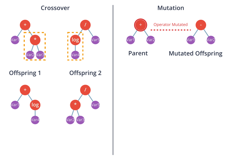
While Deep Feature Synthesis provides a structured, exhaustive approach to feature generation, other methods offer a more dynamic and optimization-driven strategy. Genetic Programming (GP) is a prominent example from the field of evolutionary computation. GP treats the problem of finding the best features as an optimization problem solved through principles inspired by biological evolution. In this paradigm, a “feature” is represented as a tree structure, where the internal nodes are mathematical operators (primitives like +, -, *, /, sin, log) and the leaf nodes are the raw input variables from the dataset. This tree structure is directly analogous to an executable program or a mathematical formula.
The GP algorithm begins by creating an initial population of these feature-trees, typically generated randomly. Each tree in the population represents a candidate feature. The algorithm then enters an iterative evolutionary loop:
- Fitness Evaluation: Each feature-tree in the population is evaluated based on its “fitness.” In the context of feature engineering, fitness is typically measured by how well the feature improves the performance of a chosen machine learning model (e.g., by measuring the increase in AUC, accuracy, or reduction in log-loss when the feature is added to the model). This evaluation is the most computationally expensive part of the process.
- Selection: The fittest individuals (the best features) are selected to “reproduce” and pass their characteristics to the next generation. This is often done using methods like tournament selection, where small random subsets of the population “compete,” and the winner proceeds.
- Reproduction: New features for the next generation are created using genetic operators:
- Crossover: Two parent trees are selected, and a random subtree from each is swapped to create two new offspring trees. This mimics the exchange of genetic material in biological reproduction and allows the algorithm to combine good “building blocks” from different successful features.
- Mutation: A random part of a single parent tree is altered. For example, an operator node might be changed (e.g.,
+becomes*), or a leaf node might be swapped for a different input variable. Mutation introduces new genetic material into the population, preventing premature convergence to a suboptimal solution.
This cycle of evaluation, selection, and reproduction continues for a set number of generations or until the fitness of the population plateaus. The final output is the best feature-tree (or set of trees) discovered during the evolutionary process. GP’s key advantage is its flexibility; it is not constrained by a predefined set of feature templates like DFS. It can discover complex, non-linear interactions that might be missed by other methods. However, this flexibility comes at a cost: GP is computationally intensive, can be prone to overfitting by creating overly complex features, and its stochastic nature means results may not be perfectly reproducible across runs.
flowchart TD
    A[Start] --> B[Initialize Population<br/>Create random feature combinations<br/>and transformations]

    B --> C[Evaluate Fitness<br/>Test each feature set on<br/>validation data using ML model]

    C --> D{Termination<br/>Criteria Met?<br/>Max generations or<br/>fitness threshold}

    D -->|No| E[Selection<br/>Choose best performing<br/>feature sets as parents<br/>using tournament/roulette]

    E --> F[Crossover & Mutation<br/>Combine parent features<br/>and apply random changes<br/>to create offspring]

    F --> G[New Population<br/>Replace old generation<br/>with offspring, keep<br/>some elite solutions]

    G --> C

    D -->|Yes| H[Return Best Features<br/>Output the highest fitness<br/>feature set discovered]

    H --> I[End]

    style A fill:#e1f5fe
    style I fill:#e8f5e8
    style D fill:#fff3e0
    style H fill:#f3e5f5
Managing Complexity and the Feature Explosion
A significant challenge in automated feature engineering is managing the sheer volume of generated features, often referred to as the feature explosion. An automated system can easily generate millions of candidate features, most of which will be redundant, irrelevant, or noisy. Using this massive feature set directly in a model would lead to several problems: increased training time, a higher risk of overfitting (due to the curse of dimensionality), and difficulties in model interpretation and maintenance. Therefore, a critical component of any automated feature engineering pipeline is automated feature selection.
Feature selection methods are algorithms designed to identify the most valuable subset of features from a larger set. These methods can be broadly categorized into three types:
- Filter Methods: These methods rank features based on their intrinsic statistical properties, independent of any machine learning model. They are computationally efficient and serve as a good first pass to eliminate clearly irrelevant features. Common techniques include calculating the correlation with the target variable, mutual information, or statistical tests like ANOVA F-tests. For example, one might discard any feature with a correlation to the target below a certain threshold or with near-zero variance.
- Wrapper Methods: These methods use a specific machine learning model to evaluate the utility of feature subsets. They treat the feature selection problem as a search problem, where different combinations of features are used to train a model, and the combination that yields the best performance is chosen. Recursive Feature Elimination (RFE) is a classic example, where a model is trained on all features, the least important feature is removed, and the process is repeated until the desired number of features is reached. Wrapper methods are more accurate than filter methods as they account for feature interactions, but they are computationally much more expensive.
- Embedded Methods: These methods perform feature selection as an integral part of the model training process. They are a compromise between the efficiency of filter methods and the accuracy of wrapper methods. The most common examples are models that use L1 regularization (Lasso). The L1 penalty term in the model’s loss function, \(\lambda \sum_{j=1}^{p} |\beta_j|\), forces the coefficients (\(\beta_j\)) of less important features to become exactly zero, effectively performing feature selection automatically during training. Tree-based models like Random Forest and Gradient Boosting also provide intrinsic feature importance scores, which can be used to rank and select features.
graph TD
            A["<b>Generated Feature Space</b><br>(1,000,000+ Features)"]
            B["<b>Stage 1: Filter Methods</b><br><i>(e.g., Remove zero-variance & low-correlation features)</i><br><b>Goal:</b> Drastic, fast reduction"]
            C["<b>Reduced Feature Space</b><br>(~10,000 Features)"]
            D["<b>Stage 2: Embedded Methods</b><br><i>(e.g., L1 Regularization or Tree-based importance)</i><br><b>Goal:</b> Efficiently find strong signals"]
            E["<b>Candidate Feature Space</b><br>(~100-500 Features)"]
            F["<b>Stage 3: Wrapper Methods (Optional)</b><br><i>(e.g., Recursive Feature Elimination)</i><br><b>Goal:</b> Fine-tune selection for max performance"]
            G["<b>Final Production Feature Set</b><br>(10-100 Features)"]

            A --> B;
            B --> C;
            C --> D;
            D --> E;
            E --> F;
            F --> G;

            style A fill:#9b59b6,stroke:#9b59b6,stroke-width:1px,color:#ebf5ee
            style B fill:#78a1bb,stroke:#78a1bb,stroke-width:1px,color:#283044
            style C fill:#9b59b6,stroke:#9b59b6,stroke-width:1px,color:#ebf5ee
            style D fill:#78a1bb,stroke:#78a1bb,stroke-width:1px,color:#283044
            style E fill:#9b59b6,stroke:#9b59b6,stroke-width:1px,color:#ebf5ee
            style F fill:#f1c40f,stroke:#f1c40f,stroke-width:1px,color:#283044
            style G fill:#2d7a3d,stroke:#2d7a3d,stroke-width:2px,color:#ebf5eeI
In a practical workflow, these methods are often combined. A fast filter method might be used first to drastically reduce the feature space from millions to thousands. Then, an embedded or wrapper method can be applied to this reduced set to select the final, most predictive features for the production model. This multi-stage approach balances computational cost with selection accuracy, making the management of the feature explosion tractable.
Practical Examples and Implementation
Development Environment Setup
To effectively follow the implementation examples in this chapter, a modern Python environment is required. We will primarily use Python 3.11+ and rely on several key libraries. The setup can be managed using a virtual environment to avoid conflicts with system-wide packages.
Tip: Using a virtual environment manager like
venvorcondais a crucial best practice in professional Python development. It ensures project dependencies are isolated and reproducible.
First, create and activate a new virtual environment:
# Using venv (standard library)
python3 -m venv auto-fe-env
source auto-fe-env/bin/activate

# On Windows, the activation command is:
# auto-fe-env\Scripts\activate
Next, install the necessary libraries using pip. We will need featuretools for deep feature synthesis, pandas for data manipulation, scikit-learn for modeling and feature selection, matplotlib and seaborn for visualization, and composeml for handling time-series data.
pip install featuretools pandas scikit-learn matplotlib seaborn composeml
Library Overview:
- Featuretools (v1.29.0): The core library for our automated feature engineering examples. It provides a powerful API for defining entities and relationships and running Deep Feature Synthesis.
- Pandas (v2.2.2): The de facto standard for data manipulation in Python. We will use it to load, clean, and structure our data before feeding it into Featuretools.
- Scikit-learn (v1.4.2): A comprehensive machine learning library. We will use it for building predictive models, performing feature selection, and evaluating performance.
- ComposeML (v0.12.0): A library built by the same team as Featuretools, specifically designed to prevent label leakage in time-series forecasting problems by correctly handling temporal data during feature engineering.
For the dataset, we will use a simulated retail dataset, which is a common use case for automated feature engineering. You can download or generate this dataset using provided scripts. The dataset will consist of multiple related tables: customers, sessions, and transactions.
Core Implementation Examples
Let’s walk through a complete example of using Featuretools to perform Deep Feature Synthesis. Our goal is to predict which customers will make a purchase in a future time window.
1. Data Loading and Preparation
First, we load our relational data into Pandas DataFrames. It’s crucial that each DataFrame has a unique index.
import pandas as pd
import featuretools as ft

# Load the datasets
# In a real scenario, these would be loaded from a database or file system.
# Here, we create sample data for demonstration.

customers_df = pd.DataFrame({
    "customer_id": [1, 2, 3, 4],
    "signup_date": pd.to_datetime(["2024-01-01", "2024-01-15", "2024-02-10", "2024-03-01"]),
    "region": ["North", "South", "North", "East"]
})

sessions_df = pd.DataFrame({
    "session_id": range(8),
    "customer_id": [1, 2, 1, 3, 2, 4, 1, 3],
    "session_start": pd.to_datetime([
        "2024-02-01", "2024-02-12", "2024-02-15", "2024-03-05",
        "2024-03-10", "2024-04-01", "2024-04-05", "2024-04-12"
    ]),
    "device": ["Desktop", "Mobile", "Desktop", "Mobile", "Tablet", "Desktop", "Mobile", "Mobile"]
})

transactions_df = pd.DataFrame({
    "transaction_id": range(12),
    "session_id": [0, 0, 1, 2, 2, 3, 4, 4, 5, 6, 7, 7],
    "transaction_time": pd.to_datetime([
        "2024-02-01 10:05", "2024-02-01 10:07", "2024-02-12 18:30", "2024-02-15 11:00",
        "2024-02-15 11:02", "2024-03-05 09:45", "2024-03-10 20:15", "2024-03-10 20:25",
        "2024-04-01 13:00", "2024-04-05 16:50", "2024-04-12 14:10", "2024-04-12 14:11"
    ]),
    "amount": [10.50, 5.25, 120.00, 35.70, 15.00, 88.10, 45.50, 5.00, 250.00, 12.00, 75.30, 8.50]
})
2. Defining the EntitySet
The EntitySet is the central data structure in Featuretools. It’s a container for our DataFrames and the relationships between them.
# Create an EntitySet
es = ft.EntitySet(id="retail_data")

# Add entities (DataFrames) to the EntitySet
es = es.add_dataframe(
    dataframe_name="customers",
    dataframe=customers_df,
    index="customer_id",
    time_index="signup_date"
)

es = es.add_dataframe(
    dataframe_name="sessions",
    dataframe=sessions_df,
    index="session_id",
    time_index="session_start"
)

es = es.add_dataframe(
    dataframe_name="transactions",
    dataframe=transactions_df,
    index="transaction_id",
    time_index="transaction_time",
    make_index=True # make_index=True if the index is not already unique
)

# Define the relationships between entities
es = es.add_relationship("customers", "customer_id", "sessions", "customer_id")
es = es.add_relationship("sessions", "session_id", "transactions", "session_id")

print(es)
Generated feature matrix:
             COUNT(sessions)  COUNT(transactions)  ...  SUM(sessions.SKEW(transactions.amount))  SUM(sessions.STD(transactions.amount))
customer_id                                        ...
1                          3                    5  ...                                      0.0                               18.349421
2                          2                    3  ...                                      0.0                               28.637825
3                          2                    3  ...                                      0.0                               47.234733
4                          1                    1  ...                                      0.0                                0.000000

[4 rows x 56 columns]
3. Running Deep Feature Synthesis (DFS)
With the EntitySet defined, we can now run DFS to generate features for our target entity, customers. The target_dataframe_name parameter tells DFS which entity we want to build features for.
# Run DFS to generate features for the 'customers' entity
# max_depth=2 means we stack up to two primitives
feature_matrix, feature_defs = ft.dfs(
    entityset=es,
    target_dataframe_name="customers",
    agg_primitives=["sum", "mean", "std", "count", "num_unique", "mode"],
    trans_primitives=["day", "month", "weekday", "time_since_previous"],
    max_depth=2,
    verbose=1
)

# Display the resulting feature matrix
print("Generated Feature Matrix Shape:", feature_matrix.shape)
print(feature_matrix.head())
Outputs:
Generated Feature Matrix Shape: (4, 27)
             COUNT(sessions)  COUNT(transactions)  ...  SUM(sessions.STD(transactions.amount))  SUM(sessions.TIME_SINCE_PREVIOUS(session_start))
customer_id                                        ...
1                          3                    5  ...                               18.349421                                          604800.0
2                          2                    3  ...                               28.637825                                         1382400.0
3                          2                    3  ...                               47.234733                                         2246400.0
4                          1                    1  ...                                0.000000                                         1900800.0

[4 rows x 27 columns]
The feature_matrix is a Pandas DataFrame where rows correspond to customers and columns are the newly generated features. feature_defs is a list of feature objects, which are useful for understanding how each feature was created.
Some example features that might be generated:
COUNT(sessions): The total number of sessions for each customer.SUM(transactions.amount): The total amount spent by each customer.MEAN(sessions.COUNT(transactions)): The average number of transactions per session for each customer.MODE(sessions.device): The most common device used by each customer.MONTH(signup_date): The month the customer signed up.STD(sessions.TIME_SINCE_PREVIOUS(session_start)): The standard deviation of the time between a customer’s sessions.
This single command generates a rich feature set that would have taken hours or days to create manually.
Step-by-Step Tutorials
Tutorial: Handling Time-Series Data and Preventing Leakage
A critical pitfall in feature engineering for time-series problems is data leakage. This occurs when information from the future (relative to a given prediction time) is used to create features, leading to unrealistically optimistic model performance that fails in production. Featuretools and ComposeML provide robust mechanisms to prevent this.
Let’s refine our prediction problem: for each customer, we want to predict their total spending in the next 30 days. We need to generate features for each customer at multiple points in time.
import pandas as pd
import featuretools as ft
import composeml as cp

# Load the datasets
# In a real scenario, these would be loaded from a database or file system.
# Here, we create sample data for demonstration.

customers_df = pd.DataFrame({
    "customer_id": [1, 2, 3, 4],
    "signup_date": pd.to_datetime(["2024-01-01", "2024-01-15", "2024-02-10", "2024-03-01"]),
    "region": ["North", "South", "North", "East"]
})

sessions_df = pd.DataFrame({
    "session_id": range(8),
    "customer_id": [1, 2, 1, 3, 2, 4, 1, 3],
    "session_start": pd.to_datetime([
        "2024-02-01", "2024-02-12", "2024-02-15", "2024-03-05",
        "2024-03-10", "2024-04-01", "2024-04-05", "2024-04-12"
    ]),
    "device": ["Desktop", "Mobile", "Desktop", "Mobile", "Tablet", "Desktop", "Mobile", "Mobile"]
})

transactions_df = pd.DataFrame({
    "transaction_id": range(12),
    "session_id": [0, 0, 1, 2, 2, 3, 4, 4, 5, 6, 7, 7],
    "transaction_time": pd.to_datetime([
        "2024-02-01 10:05", "2024-02-01 10:07", "2024-02-12 18:30", "2024-02-15 11:00",
        "2024-02-15 11:02", "2024-03-05 09:45", "2024-03-10 20:15", "2024-03-10 20:25",
        "2024-04-01 13:00", "2024-04-05 16:50", "2024-04-12 14:10", "2024-04-12 14:11"
    ]),
    "amount": [10.50, 5.25, 120.00, 35.70, 15.00, 88.10, 45.50, 5.00, 250.00, 12.00, 75.30, 8.50]
})

# Create an EntitySet
es = ft.EntitySet(id="retail_data")

# Add entities (DataFrames) to the EntitySet
es = es.add_dataframe(
    dataframe_name="customers",
    dataframe=customers_df,
    index="customer_id",
    time_index="signup_date"
)

es = es.add_dataframe(
    dataframe_name="sessions",
    dataframe=sessions_df,
    index="session_id",
    time_index="session_start"
)

es = es.add_dataframe(
    dataframe_name="transactions",
    dataframe=transactions_df,
    index="transaction_id",
    time_index="transaction_time"
)

# Define the relationships between entities
es = es.add_relationship("customers", "customer_id", "sessions", "customer_id")
es = es.add_relationship("sessions", "session_id", "transactions", "session_id")

print("EntitySet:")
print(es)
print("\n" + "="*50 + "\n")

# Generate features using DFS
feature_matrix, feature_defs = ft.dfs(
    entityset=es,
    target_dataframe_name="customers",
    agg_primitives=["sum", "mean", "std", "count", "num_unique", "mode"],
    trans_primitives=["day", "month", "weekday", "time_since_previous"],
    max_depth=2,
    verbose=1
)

print("Generated Feature Matrix Shape:", feature_matrix.shape)
print("\nFeature Matrix:")
print(feature_matrix.head())
print(f"\nTotal features generated: {len(feature_defs)}")
print("\n" + "="*50 + "\n")

# ComposeML Label Generation
# Define a labeling function that calculates total transaction amount in the next window
def total_spent_next_window(df, **kwargs):
    """
    Calculate total amount spent by a customer in the given time window
    """
    return df['amount'].sum()

# Create the LabelMaker with correct parameters
# Note: Different versions use different parameter names
# Try the newer API first, then fall back to older versions
try:
    # For newer versions (0.9.0+)
    label_maker = cp.LabelMaker(
        target_dataframe_name="customer_id",  # The entity we're making predictions for
        time_index="transaction_time",         # Time column in the data
        labeling_function=total_spent_next_window,
        window_size="30d"  # Look forward 30 days
    )
except TypeError:
    try:
        # For older versions that use target_entity
        label_maker = cp.LabelMaker(
            target_entity="customer_id",
            time_index="transaction_time",
            labeling_function=total_spent_next_window,
            window_size="30d"
        )
    except TypeError:
        # For versions that use target_dataframe_index
        label_maker = cp.LabelMaker(
            target_dataframe_index="customer_id",
            time_index="transaction_time",
            labeling_function=total_spent_next_window,
            window_size="30d"
        )

# Create cutoff times - points in time where we want to make predictions
cutoff_times = pd.DataFrame({
    "customer_id": [1, 2, 3, 4, 1, 2, 3, 4],
    "time": pd.to_datetime(["2024-02-28"] * 4 + ["2024-03-31"] * 4)
})

print("Cutoff times:")
print(cutoff_times)
print("\n" + "="*50 + "\n")

# For ComposeML, we need to prepare the data differently
# Merge all data into a single dataframe
merged_data = transactions_df.merge(sessions_df, on='session_id').merge(customers_df, on='customer_id')
merged_data = merged_data.sort_values('transaction_time')

print("Merged data for ComposeML:")
print(merged_data.head())
print("\n" + "="*50 + "\n")

# Method 1: Using ComposeML search (if it works with your version)
try:
    labels = label_maker.search(
        merged_data,
        num_examples_per_instance=2,  # Generate 2 examples per customer
        minimum_data="1d",  # Need at least 1 day of data before making labels
        verbose=True
    )
    print("Labels generated using ComposeML:")
    print(labels.head(10))
except Exception as e:
    print(f"ComposeML search failed: {e}")
    print("Using alternative manual approach...")

    # Method 2: Manual label generation as alternative
    labels_list = []

    for _, row in cutoff_times.iterrows():
        customer_id = row['customer_id']
        cutoff_time = row['time']
        window_end = cutoff_time + pd.Timedelta('30d')

        # Get transactions for this customer in the window
        customer_transactions = merged_data[
            (merged_data['customer_id'] == customer_id) &
            (merged_data['transaction_time'] >= cutoff_time) &
            (merged_data['transaction_time'] < window_end)
        ]

        total_spent = customer_transactions['amount'].sum() if not customer_transactions.empty else 0

        labels_list.append({
            'customer_id': customer_id,
            'time': cutoff_time,
            'total_spent_next_30d': total_spent
        })

    labels = pd.DataFrame(labels_list)
    print("Labels generated manually:")
    print(labels)

print("\n" + "="*50 + "\n")

# Now let's create features at the cutoff times for prediction
print("Creating features at cutoff times...")

# Generate features at specific cutoff times
cutoff_times_for_features = cutoff_times.copy()
cutoff_times_for_features.columns = ['customer_id', 'time']

feature_matrix_cutoff, _ = ft.dfs(
    entityset=es,
    target_dataframe_name="customers",
    cutoff_time=cutoff_times_for_features,
    agg_primitives=["sum", "mean", "count"],
    max_depth=1,
    verbose=1
)

print("Feature matrix at cutoff times:")
print(feature_matrix_cutoff.head(10))

# Combine features with labels for a complete dataset
if 'labels' in locals():
    # Reset index to get customer_id and time as columns
    feature_df = feature_matrix_cutoff.reset_index()

    # Check what columns we have
    print("Feature matrix columns after reset_index:")
    print(feature_df.columns.tolist())
    print("Feature matrix shape:", feature_df.shape)
    print("Sample rows:")
    print(feature_df.head(3))

    print("\nLabels columns:")
    print(labels.columns.tolist())
    print("Labels shape:", labels.shape)
    print("Sample labels:")
    print(labels.head(3))

    # For features generated with cutoff times, the index should contain both customer_id and time
    # Let's check if we need to handle the merge differently
    if 'time' in feature_df.columns:
        # Standard merge on both customer_id and time
        final_dataset = feature_df.merge(
            labels,
            on=['customer_id', 'time'],
            how='inner'
        )
    elif len(feature_df.index.names) == 2:
        # Multi-index case - customer_id and time are in the index
        feature_df_indexed = feature_df.set_index(['customer_id', 'time'])
        labels_indexed = labels.set_index(['customer_id', 'time'])
        final_dataset = feature_df_indexed.merge(
            labels_indexed,
            left_index=True,
            right_index=True,
            how='inner'
        ).reset_index()
    else:
        # Fallback: merge only on customer_id
        print("Warning: Merging only on customer_id as time column structure differs")
        final_dataset = feature_df.merge(
            labels,
            on='customer_id',
            how='inner'
        )

    print("\nFinal dataset with features and labels:")
    print(final_dataset.head())
    print(f"Dataset shape: {final_dataset.shape}")

    # Show feature importance (non-zero numeric features)
    # First, get all feature columns (excluding target and ID columns)
    exclude_cols = ['customer_id', 'time', 'total_spent_next_30d']
    all_feature_cols = [col for col in final_dataset.columns if col not in exclude_cols]

    # Filter for numeric columns only
    numeric_feature_cols = []
    categorical_feature_cols = []

    for col in all_feature_cols:
        try:
            # Try to sum - if it works, it's numeric
            _ = final_dataset[col].sum()
            if final_dataset[col].sum() != 0:  # Only include non-zero features
                numeric_feature_cols.append(col)
        except (TypeError, AttributeError):
            # If sum fails, it's categorical
            categorical_feature_cols.append(col)

    print(f"\nNumeric features with non-zero values ({len(numeric_feature_cols)}):")
    for col in numeric_feature_cols[:10]:  # Show first 10
        try:
            mean_val = final_dataset[col].mean()
            print(f"  {col}: {mean_val:.2f} (avg)")
        except:
            print(f"  {col}: (unable to calculate mean)")

    print(f"\nCategorical features ({len(categorical_feature_cols)}):")
    for col in categorical_feature_cols[:5]:  # Show first 5
        unique_vals = final_dataset[col].nunique()
        print(f"  {col}: {unique_vals} unique values")

    print(f"\nTotal features: {len(all_feature_cols)} (numeric: {len(numeric_feature_cols)}, categorical: {len(categorical_feature_cols)})")
else:
    print("No labels were generated successfully.")
The cutoff_times DataFrame is the key to preventing leakage. When we run DFS with these cutoff times, Featuretools will ensure that for each row (i.e., for each prediction at a specific time), only data available before that cutoff time is used for feature calculation.
# Now, run DFS using the cutoff times to generate time-aware features
feature_matrix_time_aware = ft.calculate_feature_matrix(
    features=feature_defs,  # Use the same feature definitions from before
    entityset=es,
    cutoff_time=labels[['customer_id', 'time']],  # DataFrame with instance_id and time columns
    verbose=True,
    include_cutoff_time=True  # New parameter in latest version (default True)
)

# The resulting feature matrix is now aligned with our labels and is leakage-free.
# We can merge it with the labels to create our final training set.

# Debug: Check the structure of both dataframes
print("Feature matrix info:")
print("Shape:", feature_matrix_time_aware.shape)
print("Index:", feature_matrix_time_aware.index.names)
print("Index type:", type(feature_matrix_time_aware.index))
print("Sample index values:")
print(feature_matrix_time_aware.index[:5])

print("\nLabels info:")
print("Shape:", labels.shape)
print("Columns:", labels.columns.tolist())
print("Sample labels:")
print(labels.head())

# Always reset index to avoid join issues
feature_matrix_reset = feature_matrix_time_aware.reset_index()
print("\nFeature matrix after reset_index:")
print("Columns:", feature_matrix_reset.columns.tolist())
print("Sample rows:")
print(feature_matrix_reset.head(3))

# Create a robust merge approach
try:
    # Method 1: Try direct merge on common columns
    common_cols = list(set(feature_matrix_reset.columns) & set(labels.columns))
    print(f"\nCommon columns for merge: {common_cols}")

    if len(common_cols) >= 1:
        training_data = feature_matrix_reset.merge(
            labels,
            on=common_cols,
            how='inner'
        )
        print(f"Merge successful using columns: {common_cols}")
    else:
        raise ValueError("No common columns found")

except Exception as e:
    print(f"Direct merge failed: {e}")

    # Method 2: Manual alignment approach
    print("Attempting manual alignment...")

    # Ensure both dataframes have the same key columns
    if 'customer_id' in feature_matrix_reset.columns and 'customer_id' in labels.columns:
        # Add row numbers to help with alignment
        feature_matrix_reset = feature_matrix_reset.reset_index(drop=True)
        labels_reset = labels.reset_index(drop=True)

        # Create a combined key for matching
        if 'time' in feature_matrix_reset.columns and 'time' in labels_reset.columns:
            feature_matrix_reset['merge_key'] = (
                feature_matrix_reset['customer_id'].astype(str) + "_" +
                feature_matrix_reset['time'].astype(str)
            )
            labels_reset['merge_key'] = (
                labels_reset['customer_id'].astype(str) + "_" +
                labels_reset['time'].astype(str)
            )

            training_data = feature_matrix_reset.merge(
                labels_reset,
                on='merge_key',
                how='inner',
                suffixes=('', '_label')
            ).drop('merge_key', axis=1)
        else:
            # Fallback: merge only on customer_id
            training_data = feature_matrix_reset.merge(
                labels_reset,
                on='customer_id',
                how='inner',
                suffixes=('', '_label')
            )
    else:
        print("Error: Cannot find customer_id column in both dataframes")
        training_data = None

if training_data is not None:
    print("\nTraining data created successfully!")
    print("Training data shape:", training_data.shape)
    print("Training data columns:", training_data.columns.tolist())
    print("\nTraining data sample:")
    print(training_data.head())

    # Clean up duplicate columns if any
    duplicate_cols = [col for col in training_data.columns if col.endswith('_label')]
    if duplicate_cols:
        print(f"\nRemoving duplicate columns: {duplicate_cols}")
        training_data = training_data.drop(duplicate_cols, axis=1)
else:
    print("Failed to create training data")
This disciplined, time-aware approach is essential for building models that generalize well to unseen data in a production time-series setting.
Integration and Deployment Examples
Once a feature matrix is generated and a model is trained, the feature engineering logic must be integrated into the production prediction pipeline. This means that when a new prediction is requested for a customer, the same feature generation process must be applied using the most up-to-date data.
Featuretools facilitates this by allowing you to save feature definitions.
# Save the feature definitions to a file
ft.save_features(feature_defs, "my_feature_definitions.json")

# In a production environment, load the definitions
loaded_feature_defs = ft.load_features("my_feature_definitions.json")

# When a new prediction is needed for customer_id=1 today:
# 1. Update the EntitySet with the latest data from the production database.
# 2. Create a cutoff time for the prediction.
prediction_cutoff = pd.DataFrame({
    "customer_id": [1],
    "time": [pd.Timestamp.now(tz="UTC")]
})

# 3. Calculate the feature vector for this specific instance.
feature_vector = ft.calculate_feature_matrix(
    features=loaded_feature_defs,
    entityset=es, # The updated EntitySet
    cutoff_time=prediction_cutoff
)

# 4. Use the trained model to make a prediction.
# model.predict(feature_vector)
This workflow ensures that the features used for inference are created in exactly the same way as the features used for training, which is critical for model consistency and performance. In a full MLOps pipeline, this process would be orchestrated by a tool like Kubeflow Pipelines or Airflow, which would trigger data updates, feature calculation, and model prediction on a schedule or via an API call.
Warning: Mismatches between the training and inference feature generation logic, known as training-serving skew, are a common and severe source of error in production ML systems. Versioning feature definitions and using a centralized feature store are best practices to mitigate this risk.
Industry Applications and Case Studies
The adoption of automated feature engineering is accelerating across various industries, driven by the need to extract more value from complex data assets and to shorten development cycles.
- E-commerce and Retail: Companies like Wayfair and Instacart use automated feature engineering to predict customer lifetime value (CLV), churn, and product recommendations. By analyzing vast streams of transactional and behavioral data (clicks, page views, add-to-carts), they can generate thousands of features that capture subtle user behaviors. For example, features like “average time between sessions” or “standard deviation of purchase value in the last 90 days” can be highly predictive of churn. The business impact is significant, leading to more effective marketing campaigns, personalized user experiences, and improved inventory management. The main challenge is handling the sheer volume and velocity of the data and ensuring feature calculations are performed efficiently at scale.
- Financial Services: In finance, automated feature engineering is applied to fraud detection, credit scoring, and algorithmic trading. For a credit scoring model, an automated system can analyze a customer’s transaction history, loan payments, and account interactions to generate features that signal creditworthiness. For instance, a feature like
NUM_UNIQUE(merchants where SUM(transactions.amount) > 1000)could indicate diverse spending habits. The key challenge in this domain is model interpretability. Regulators often require financial institutions to explain their model’s decisions, which can be difficult when using thousands of complex, automatically generated features. This has led to research into combining automated feature generation with interpretable modeling techniques. - Healthcare and Life Sciences: Researchers and providers use these techniques to predict disease progression, patient risk, and treatment efficacy from electronic health records (EHR). EHR data is notoriously complex and multi-relational (patients, diagnoses, medications, lab results). Automated feature engineering can systematically explore this data to uncover novel biomarkers or risk factors. A feature like
STD(lab_results.glucose_level where time > 6 months ago)could be a powerful predictor for diabetes onset. The primary constraints are data privacy (HIPAA compliance) and the need for rigorous validation, as model errors can have severe consequences. - Industrial IoT (Internet of Things): In manufacturing and energy, automated feature engineering is used for predictive maintenance. Sensor data from machinery (temperature, pressure, vibration) is collected at high frequency. Automated systems can generate features from these time-series signals, such as rolling averages, frequency-domain features (via Fourier transforms), or the time since the last anomalous reading. These features are then used to predict equipment failure before it occurs, saving millions in downtime and repair costs. The challenge is the massive scale of time-series data and the need for real-time feature computation for immediate alerting.
Best Practices and Common Pitfalls
Successfully integrating automated feature engineering into a production workflow requires discipline and adherence to best practices. Simply generating millions of features is not a silver bullet and can introduce new problems if not managed carefully.
- Start with Domain Knowledge, Then Automate: Automated tools are most effective when guided by human expertise. Before running DFS or GP, collaborate with domain experts to define the core entities, relationships, and potentially valuable custom primitives. This hybrid approach, combining human intuition with algorithmic scale, often yields the best results. Don’t treat the process as a complete black box.
- Rigorously Manage Data Leakage: As highlighted in the practical examples, temporal data leakage is the most common and dangerous pitfall. Always use point-in-time validation strategies. When defining a prediction problem, clearly state the “time of prediction” and ensure no data from after this point is used to construct features or labels. Tools like Featuretools’
cutoff_timeare designed for this, but the conceptual discipline must be maintained by the engineer. - Invest in a Robust Feature Selection Strategy: Do not feed all generated features into your model. This leads to overfitting, long training times, and complex, unmaintainable models. Implement a multi-stage feature selection pipeline. Use computationally cheap filter methods to perform an initial culling, followed by more sophisticated embedded or wrapper methods. The goal is to find the smallest set of features that provides the best model performance.
- Think About “Feature Interpretability”: While not all models require interpretation, many business-critical applications do (e.g., finance, healthcare). The features generated by DFS are often quite interpretable because their derivation is explicitly tracked (e.g.,
MEAN(sessions.COUNT(transactions))). Features from GP can be much more opaque. Document and review the top features selected for your model. If they are not understandable, it could indicate a problem with the data or the generation process. - Monitor Feature Distributions in Production: Data distributions can and do change over time, a phenomenon known as data drift. A feature that was predictive during training may become less so in production. Implement monitoring systems that track the statistical properties (mean, variance, null rate) of your model’s features over time. Set up alerts for when these distributions drift significantly, as this may signal that the model needs to be retrained.
- Consider the Computational Cost: Generating a massive feature matrix can be computationally expensive and time-consuming. Profile your feature generation process. Can some features be pre-computed and stored in a feature store? Can the computation be distributed using frameworks like Dask or Spark? Optimize the process to meet the latency requirements of your application (batch vs. real-time).
Hands-on Exercises
- Basic: Exploring Feature Primitives:
- Objective: Understand the difference between aggregation and transformation primitives.
- Task: Using the retail dataset from the implementation section, manually define and list five potentially useful transformation primitives that could be applied to the
transactionsorsessionstables (e.g.,is_weekend,log_amount). Then, define and list five aggregation primitives that could be used to summarizetransactionsfor eachsession. - Verification: Run
ft.list_primitives()to see the built-in primitives in Featuretools and compare them to your list. Explain why each of your chosen primitives might be useful.
- Intermediate: Custom Feature Primitives:
- Objective: Extend Featuretools with domain-specific knowledge.
- Task: The
amountcolumn in ourtransactionsdata is skewed. A common transformation for skewed financial data is the Box-Cox transformation. Research and implement a custom Featuretools transformation primitive for the Box-Cox transformation (you can usescipy.stats.boxcox). Apply this custom primitive during DFS and see if it appears in the generated feature list. - Hint: You will need to define a Python function and use the
@featuretools.primitives.make_trans_primitivedecorator. - Success Criteria: Successfully run DFS with your custom primitive and identify a generated feature that uses it.
- Advanced: End-to-End Modeling and Feature Selection:
- Objective: Build a complete prediction pipeline, from feature generation to model training and evaluation, including feature selection.
- Task:
- Using the time-aware feature matrix and labels generated in the tutorial, split the data into a training and a testing set based on time (e.g., use the first cutoff time for training, the second for testing).
- Train a baseline
LogisticRegressionmodel on the raw (non-generated) customer features. - Train another
LogisticRegressionmodel on the full, automatically generated feature set. Compare the performance (e.g., AUC). - Implement a feature selection step. Use
sklearn.feature_selection.SelectFromModelwith aRandomForestClassifierto select the top 20 features from the full set. - Train a final
LogisticRegressionmodel on only these 20 selected features.
- Expected Outcome: Compare the performance, training time, and number of features for all three models. You should find that the model with automated features outperforms the baseline, and the model with selected features performs comparably to the full model but is much simpler.
- Team-Based: Genetic Programming Challenge:
- Objective: Explore feature discovery using an evolutionary approach.
- Task: Using a library like
gplearn, attempt to solve the same prediction problem. Configure the GP regressor to discover the best feature formula to predict customer spending. - Guidance: Divide tasks among the team: one person can handle data preparation, another can configure the GP parameters (population size, generations, function set), and a third can analyze the results.
- Verification: Present the best formula discovered by the GP algorithm. Analyze its complexity and compare its performance to the features generated by Featuretools. Discuss the pros and cons of the GP approach you observed.
Tools and Technologies
- Featuretools: The leading open-source library for automated feature engineering using Deep Feature Synthesis. Its core strength lies in its intuitive API for handling multi-table, relational, and temporal data. It is built on top of Pandas and integrates well with the Dask for parallel computation.
- ComposeML: A companion library to Featuretools, specifically designed for structuring and labeling time-series prediction problems in a way that prevents data leakage. It simplifies the process of generating time-aware training examples.
- gplearn: A popular Python library for implementing genetic programming. It is compliant with the scikit-learn API, making it easy to integrate into existing ML workflows for symbolic regression and classification tasks. It’s a great tool for exploring the evolutionary approach to feature discovery.
- scikit-learn: While not a feature generation tool itself, its feature selection module (
sklearn.feature_selection) is an indispensable part of any automated feature engineering pipeline for managing the feature explosion. - Feature Stores (e.g., Tecton, Feast): For production-grade MLOps, feature stores are becoming essential. They are centralized platforms for storing, serving, and managing ML features. They solve problems like training-serving skew, enable feature reuse across different models, and handle point-in-time correctness for feature retrieval. While we did not implement one here, understanding their role is crucial for deploying automated feature engineering at scale.
Summary
- Manual feature engineering is a bottleneck: It is time-consuming, not scalable, and dependent on domain expertise, making it difficult to manage in modern ML systems.
- Automation provides a systematic solution: Automated feature engineering uses algorithms to systematically search for predictive features, increasing efficiency, reproducibility, and the potential to uncover hidden patterns.
- Deep Feature Synthesis (DFS) is a core technique: DFS uses feature primitives (transformations and aggregations) and stacks them to build complex features from relational data, as implemented in libraries like Featuretools.
- Genetic Programming (GP) offers a flexible alternative: GP evolves mathematical formulas as features, providing a powerful method for discovering complex, non-linear relationships, though it can be computationally expensive.
- Managing the feature explosion is critical: The generation of millions of features necessitates a robust feature selection strategy (using filter, wrapper, or embedded methods) to avoid overfitting and reduce model complexity.
- Preventing data leakage is paramount: In time-series applications, using point-in-time correct feature generation (e.g., with
cutoff_time) is non-negotiable for building models that perform reliably in production. - Productionizing requires careful integration: The feature generation logic must be versioned and consistently applied in both training and inference pipelines, often orchestrated with MLOps tools and feature stores.
Further Reading and Resources
- Featuretools Official Documentation: The most comprehensive resource for learning the Featuretools library, with detailed tutorials and API references. (https://featuretools.alteryx.com/en/stable/)
- “Feature Engineering for Machine Learning” by Alice Zheng & Amanda Casari (O’Reilly, 2018): While not exclusively about automation, this book provides an excellent foundation on the principles of feature engineering, which is essential context.
- The Feast Tecton Blog: An industry-leading blog on the practical challenges of operationalizing machine learning, with a strong focus on feature stores and production-grade feature engineering. (https://www.tecton.ai/blog/)
- gplearn Official Documentation: The go-to guide for implementing genetic programming for feature discovery in Python. (https://gplearn.readthedocs.io/)
- Koza, J. R. (1992). Genetic Programming: On the Programming of Computers by Means of Natural Selection. (MIT Press). The foundational text on Genetic Programming, providing deep theoretical background.
- “An Introduction to Feature Extraction” – A tutorial on Kaggle: A practical, code-first introduction to various feature engineering and selection techniques. (https://www.kaggle.com/code/kanncaa1/feature-engineering-and-data-visualization)
Glossary of Terms
- Automated Feature Engineering: The process of using algorithms to automatically generate and select predictive features from raw data, reducing the need for manual, domain-expert-driven feature creation.
- Deep Feature Synthesis (DFS): An algorithm that systematically stacks feature primitives to generate a large number of complex features from relational datasets.
- EntitySet: A data structure used in Featuretools to represent a collection of data tables (entities) and the relationships between them.
- Feature Primitive: A basic, well-defined operation used to create features. They are categorized as transformation primitives (acting on a single table) and aggregation primitives (summarizing across related tables).
- Feature Store: A centralized platform in an MLOps stack for storing, managing, versioning, and serving features for both model training and real-time inference.
- Genetic Programming (GP): An evolutionary computation technique that evolves computer programs or mathematical expressions (in this context, features) to solve a problem.
- Data Leakage (Temporal Leakage): The error of using information from the future to generate features for a prediction at a point in the past. It leads to overly optimistic model performance that is not replicated in production.
- Training-Serving Skew: A discrepancy between the data processing or feature engineering logic used during model training and the logic used during model serving (inference), leading to poor production performance.
