
Chapter 9: Advanced Matrix Operations and Decomposition
Chapter Objectives
Upon successful completion of this chapter, you will be able to:
- Understand the theoretical principles behind matrix decomposition techniques, including LU, QR, and Cholesky factorization.
- Analyze the computational complexity and numerical stability of different decomposition algorithms and select the appropriate method for a given problem.
- Implement matrix decomposition algorithms from scratch and utilize optimized library functions in Python with NumPy and SciPy.
- Apply these decomposition techniques to solve practical problems in machine learning, such as solving systems of linear equations, optimizing least squares problems, and sampling from multivariate normal distributions.
- Design efficient computational workflows that leverage matrix factorization to accelerate model training and data analysis tasks.
- Evaluate the trade-offs between different decomposition methods in the context of real-world AI systems, considering factors like matrix sparsity, size, and conditioning.
Introduction
In the landscape of modern artificial intelligence, linear algebra serves as the bedrock upon which sophisticated algorithms are built. While previous chapters established fundamental concepts like vectors, matrices, and basic operations, this chapter delves into a more powerful and nuanced set of tools: matrix decomposition, also known as matrix factorization. These techniques are the computational workhorses that enable the efficient and stable solution of complex problems that are ubiquitous in machine learning, from training deep neural networks to building recommendation systems. At its core, matrix decomposition is the process of breaking down a matrix into a product of simpler, constituent matrices with desirable properties, such as being triangular, orthogonal, or diagonal. This process is analogous to factoring a composite number into its prime components; it reveals the intrinsic structure of the original matrix, making it easier to manipulate and analyze.
The importance of these methods cannot be overstated. Consider the fundamental task of solving a large system of linear equations, a problem that arises in everything from linear regression to the optimization of network flows. A naive approach using matrix inversion is often computationally prohibitive and numerically unstable. However, by decomposing the system’s matrix using a technique like LU decomposition, we can transform the problem into one that is solved rapidly and accurately. Similarly, QR decomposition is central to solving the least-squares problems that underpin regression analysis and data fitting, while Cholesky decomposition provides an incredibly efficient way to work with the covariance matrices found in Gaussian processes and Bayesian inference. This chapter will not only explore the elegant mathematics behind these techniques but will also ground them in practical, hands-on implementations, preparing you to leverage them effectively in building robust and scalable AI systems.
Technical Background
The journey into advanced matrix operations begins with understanding that a matrix is more than just a grid of numbers; it is a representation of a linear transformation. Matrix decompositions are powerful techniques for re-representing these transformations in ways that expose their fundamental geometric and algebraic properties. By breaking a complex matrix \(A\) into a product of simpler matrices, such as \(A = LU\) or \(A = QR\), we unlock computationally efficient and numerically stable methods for solving a wide range of problems that are otherwise intractable. This section lays the theoretical groundwork for the most critical decomposition techniques used in AI and machine learning.
Fundamental Concepts in Matrix Factorization
Before we explore specific algorithms, it’s crucial to grasp the core idea that unites them. The central theme is the transformation of a general matrix into matrices with specific, useful structures. The primary structures we seek are triangular, orthogonal, and diagonal matrices.
A triangular matrix is one where all entries are zero either above (lower triangular) or below (upper triangular) the main diagonal. The primary advantage of this structure is the ease with which it allows us to solve systems of linear equations. For a system \(Lx = b\), where \(L\) is lower triangular, we can find the solution \(x\) using a simple process called forward substitution. Similarly, for an upper triangular system \(Ux = b\), we use back substitution. Both processes are computationally inexpensive, with a complexity of \(O(n^2)\), a significant improvement over the \(O(n^3)\) complexity of general matrix inversion.
An orthogonal matrix \(Q\) is a square matrix whose columns and rows are orthonormal vectors. This means that \(Q^T Q = QQ^T = I\), where \(I\) is the identity matrix. The defining property of an orthogonal matrix is that it preserves the Euclidean norm, or length, of vectors it transforms; that is, \(||Qx|| = ||x||\). Geometrically, orthogonal transformations correspond to rotations and reflections. Computationally, their most valuable property is that their inverse is simply their transpose (\(Q^{-1} = Q^T\)), making inversion a trivial and numerically stable operation.
| Decomposition | Form | Matrix Requirements | Primary Use Case | Key Benefit |
|---|---|---|---|---|
| LU Decomposition | PA = LU | Square matrix | Solving Ax = b efficiently | Fast solution for multiple b vectors |
| QR Decomposition | A = QR | Any m x n matrix | Least squares problems (min ||Ax-b||) | Numerically stable |
| Cholesky Decomposition | A = LLT | Symmetric, positive definite | Covariance matrix operations | Extremely fast (~2x faster than LU) |
A diagonal matrix \(D\) is a matrix where all off-diagonal elements are zero. These are the simplest matrices to work with. Their eigenvalues are the diagonal entries, and their powers \(D^k\) are found by simply raising the diagonal entries to the \(k\)-th power. The ultimate goal of many decomposition techniques, such as eigendecomposition, is to represent a matrix in terms of a diagonal matrix, effectively simplifying its action to simple scaling along principal axes.

Solving Linear Systems: A New Perspective
The canonical problem \(Ax = b\), where we must solve for the vector \(x\), is central to countless applications. If we can decompose \(A\) into a product of two matrices, say \(A = BC\), the problem becomes \(BCx = b\). We can then solve this in two simpler steps: first, solve \(By = b\) for an intermediate vector \(y\), and then solve \(Cx = y\) for our final solution \(x\). This strategy is only effective if solving for \(y\) and \(x\) is significantly easier than solving the original system directly. This is precisely the advantage that LU, QR, and Cholesky decompositions provide. They transform a single, difficult problem into a sequence of tractable ones.
graph TD
    subgraph "Strategy: Solve Ax = b"
        A[Start: Difficult Problem <br> <b>Ax = b</b>] --> B(1- Decompose A into simpler matrices <br> <b>A = BC</b>);
        B --> C(2- Substitute into original equation <br> <b>BCx = b</b>);
        C --> D{3- Solve in two easier steps};
        D -- "Step 3a" --> E(Solve <b>By = b</b> for intermediate vector <i>y</i>);
        D -- "Step 3b" --> F(Solve <b>Cx = y</b> for final solution <b>x</b>);
        E --> F;
        F --> G[End: Solution <b>x</b>];
    end

    style A fill:#e74c3c,stroke:#e74c3c,stroke-width:2px,color:#ebf5ee
    style B fill:#78a1bb,stroke:#78a1bb,stroke-width:1px,color:#283044
    style C fill:#78a1bb,stroke:#78a1bb,stroke-width:1px,color:#283044
    style D fill:#f39c12,stroke:#f39c12,stroke-width:1px,color:#283044
    style E fill:#9b59b6,stroke:#9b59b6,stroke-width:1px,color:#ebf5ee
    style F fill:#9b59b6,stroke:#9b59b6,stroke-width:1px,color:#ebf5ee
    style G fill:#2d7a3d,stroke:#2d7a3d,stroke-width:2px,color:#ebf5ee
LU Decomposition: The Gaussian Elimination Workhorse
The LU decomposition is arguably the most fundamental matrix factorization, as it is a direct programmatic expression of the method of Gaussian elimination, which students often learn to perform by hand. It factorizes a square matrix \(A\) into the product of a lower triangular matrix \(L\) and an upper triangular matrix \(U\), such that \(A = LU\).
The Algorithm and Its Mathematical Roots
Gaussian elimination systematically transforms a matrix \(A\) into an upper triangular matrix \(U\) by applying a sequence of elementary row operations. These operations involve subtracting a multiple of one row from another to introduce zeros below the diagonal. For example, to eliminate the entry \(a_{21}\), we subtract \((a_{21}/a_{11})\) times the first row from the second row. Each of these elementary operations can be represented by multiplication with a special type of lower triangular matrix called an atomic lower triangular matrix.
If we denote the sequence of these operations as \(E_k, \dots, E_2, E_1\), then \(U = E_k \dots E_2 E_1 A\). Rearranging this gives \(A = (E_1^{-1} E_2^{-1} \dots E_k^{-1}) U\). The remarkable result is that the product of the inverses of these atomic matrices is itself a lower triangular matrix, which we call \(L\). The entries of \(L\) are simply the multipliers used during the elimination process. Specifically, the entry \(l_{ij}\) is the multiple of row \(j\) that was subtracted from row \(i\) to create a zero. \(L\) is constructed to have ones on its diagonal.
This process, however, has a critical failure point: if a pivot element \(a_{kk}\) (the diagonal element used for elimination in step \(k\)) is zero or very close to zero, the required multiplier becomes infinite or numerically unstable. This necessitates pivoting, which involves swapping rows to ensure the largest possible pivot element is used. This leads to the more general form of the decomposition: \(PA = LU\), where \(P\) is a permutation matrix that represents the row swaps.
graph TD
    subgraph LU Decomposition Flow
        A[Start: Input Matrix A, Vector b] --> B{Loop k = 1 to n-1};
        B --> C{"Find pivot: max |A(i,k)| for i >= k"};
        C --> D{Swap row k with pivot row};
        D --> E[Update Permutation Matrix P];
        E --> F{Loop i = k+1 to n};
        F --> G["Calculate multiplier L(i,k) = A(i,k)/A(k,k)"];
        G --> H["Update row i: A(i,:) -= L(i,k) * A(k,:)"];
        H --> F;
        F --> B;
        B --> I[End Loop: Output P, L, U];
    end
    subgraph "Solving Ax=b"
        J[Solve PAx = Pb] --> K[1- Apply Permutation: y = Pb];
        K --> L[2- Forward Substitution: Lz = y];
        L --> M[3- Back Substitution: Ux = z];
        M --> N[End: Solution x];
    end
    I --> J;
    style A fill:#283044,stroke:#283044,stroke-width:2px,color:#ebf5ee
    style B fill:#f39c12,stroke:#f39c12,stroke-width:1px,color:#283044
    style C fill:#78a1bb,stroke:#78a1bb,stroke-width:1px,color:#283044
    style D fill:#78a1bb,stroke:#78a1bb,stroke-width:1px,color:#283044
    style E fill:#9b59b6,stroke:#9b59b6,stroke-width:1px,color:#ebf5ee
    style F fill:#f39c12,stroke:#f39c12,stroke-width:1px,color:#283044
    style G fill:#78a1bb,stroke:#78a1bb,stroke-width:1px,color:#283044
    style H fill:#78a1bb,stroke:#78a1bb,stroke-width:1px,color:#283044
    style I fill:#2d7a3d,stroke:#2d7a3d,stroke-width:2px,color:#ebf5ee
    style J fill:#283044,stroke:#283044,stroke-width:2px,color:#ebf5ee
    style K fill:#78a1bb,stroke:#78a1bb,stroke-width:1px,color:#283044
    style L fill:#78a1bb,stroke:#78a1bb,stroke-width:1px,color:#283044
    style M fill:#78a1bb,stroke:#78a1bb,stroke-width:1px,color:#283044
    style N fill:#2d7a3d,stroke:#2d7a3d,stroke-width:2px,color:#ebf5ee
Applications and Complexity
Once \(A\) is factorized into \(PA = LU\), solving \(Ax = b\) becomes \(LUx = Pb\). This is solved in three steps:
- Apply permutations: \(y = Pb\).
- Forward substitution: Solve \(Lz = y\) for \(z\).
- Back substitution: Solve \(Ux = z\) for \(x\).
The primary cost is the initial decomposition, which has a computational complexity of \(O(n^3)\). However, once the decomposition is computed, solving for different vectors \(b\) only requires the substitution steps, which are \(O(n^2)\). This makes LU decomposition extremely efficient when solving a system with the same matrix \(A\) but multiple right-hand sides, a common scenario in iterative methods and engineering simulations. Another key application is computing the determinant of \(A\), which is simply the product of the diagonal elements of \(U\) (with a sign change depending on the number of row swaps in \(P\)).
QR Decomposition: The Orthogonal Approach
While LU decomposition is built on Gaussian elimination, QR decomposition is built on a different, geometrically-motivated process: Gram-Schmidt orthogonalization. It factorizes any \(m \times n\) matrix \(A\) into the product of an \(m \times m\) orthogonal matrix \(Q\) and an \(m \times n\) upper triangular matrix \(R\), such that \(A = QR\).
Gram-Schmidt and Numerical Stability
The classical Gram-Schmidt process provides an intuitive way to understand QR decomposition. It takes a set of linearly independent vectors (the columns of \(A\)) and generates an orthonormal set (the columns of \(Q\)) that spans the same subspace. The process works iteratively. The first column of \(Q\), \(q_1\), is a normalized version of the first column of \(A\), \(a_1\). The second vector, \(q_2\), is found by taking \(a_2\), subtracting its projection onto \(q_1\), and then normalizing the result. This continues, with each new vector \(q_k\) being made orthogonal to all previous vectors \(q_1, \dots, q_{k-1}\). The coefficients of these projections and the normalization factors form the entries of the upper triangular matrix \(R\).
However, the classical Gram-Schmidt process is known to be numerically unstable. Small floating-point errors in the subtraction steps can lead to a loss of orthogonality in the resulting \(Q\) vectors. A more robust alternative is the Modified Gram-Schmidt algorithm, which reorders the operations to improve stability. Even better are methods based on Householder reflections. A Householder transformation is a reflection about a plane that can be used to selectively introduce zeros into a vector. By applying a sequence of these reflections, we can systematically transform the columns of \(A\) into an upper triangular form \(R\). The product of these Householder matrices forms the orthogonal matrix \(Q\). This is the standard method used in high-quality numerical software.
Note: While Gram-Schmidt is easier to understand conceptually, Householder reflections are the industry standard for QR decomposition due to their superior numerical stability.
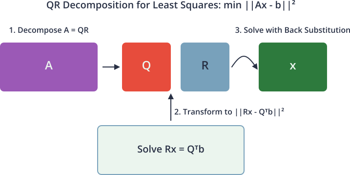
The Power of QR in Least Squares
The premier application of QR decomposition is in solving linear least squares problems. In many real-world scenarios, the system \(Ax = b\) has no exact solution because the vector \(b\) does not lie in the column space of \(A\). This is typical in regression, where measurement errors and model imperfections mean the data points do not fall perfectly on a line. The goal is instead to find the vector \(x\) that minimizes the squared Euclidean norm of the residual error:
\[\min_{x} ||Ax – b||2^2\]
Using \(A = QR\), the problem becomes:
\[\min{x} ||QRx – b||_2^2\]
Since \(Q\) is orthogonal, multiplying by \(Q^T\) does not change the norm of the residual:
\[||Q^T(QRx – b)||_2^2 = ||Rx – Q^T b||_2^2\]
Let \(Q^T b = \begin{bmatrix} c_1 \ c_2 \end{bmatrix}\), where \(c_1\) has the same number of rows as \(R\). The expression to minimize becomes:
\[||Rx – \begin{bmatrix} c_1 \ c_2 \end{bmatrix}||_2^2\]
Because \(R\) is upper triangular, this separates into two parts: \(||R_{upper}x – c_1||_2^2 + ||c_2||2^2\). The first term can be made zero by solving the square upper triangular system \(R{upper}x = c_1\), which is easily done with back substitution. The second term, \(||c_2||_2^2\), is a constant representing the final residual error. This method is not only computationally efficient but also numerically stable, avoiding the explicit formation of \(A^T A\) which is required by the normal equations and can lead to a loss of precision.
Cholesky Decomposition: The Symmetric Specialist
For the special but important class of matrices that are symmetric and positive definite, there exists a highly efficient and stable factorization: the Cholesky decomposition. A symmetric matrix \(A\) is one where \(A = A^T\). A symmetric matrix is positive definite if the scalar \(x^T A x\) is positive for every non-zero vector \(x\). Such matrices arise frequently in machine learning, most notably as covariance matrices and Gram matrices (used in kernel methods like Support Vector Machines).
The Cholesky decomposition factorizes a symmetric positive definite matrix \(A\) into the product of a lower triangular matrix \(L\) and its transpose, \(L^T\). That is, \(A = LL^T\). This can be thought of as a special case of LU decomposition where \(U = L^T\), but it can be computed more efficiently.
Algorithm and Computational Advantages
The algorithm to compute \(L\) is straightforward. The entries \(l_{ij}\) of \(L\) can be computed directly, column by column or row by row. For example, the first element is \(l_{11} = \sqrt{a_{11}}\). The rest of the first column is \(l_{i1} = a_{i1} / l_{11}\). The process continues, with each element \(l_{ij}\) depending only on the elements in \(A\) and the previously computed elements in \(L\).
A key feature of the algorithm is that it involves taking square roots. If the matrix \(A\) is not positive definite, the algorithm will at some point attempt to take the square root of a negative number, and the decomposition will fail. This makes Cholesky decomposition an effective test for positive definiteness.
The computational advantages are significant. Cholesky decomposition requires approximately \((1/3)n^3\) floating-point operations, which is about half the cost of LU decomposition for a general matrix. Furthermore, it is inherently numerically stable without any need for pivoting.
Applications in Statistics and Optimization
The primary application of Cholesky decomposition in AI is its role in dealing with multivariate normal distributions. The probability density function of a multivariate normal distribution is defined by a mean vector \(\mu\) and a covariance matrix \(\Sigma\).
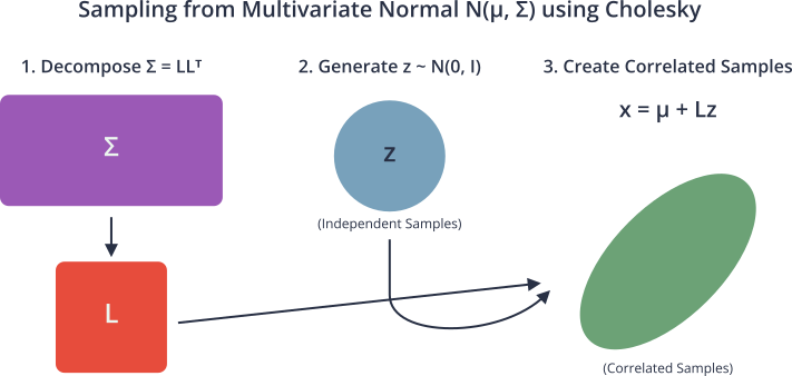
To generate random samples from this distribution, one can generate a vector \(z\) of standard independent normal random variables and then compute the sample \(x = \mu + Lz\), where \(L\) is the Cholesky factor of the covariance matrix (\(\Sigma = LL^T\)). This works because the covariance of \(Lz\) is:
\[E[(Lz)(Lz)^T] = L E[zz^T] L^T = LIL^T = LL^T = \Sigma\]
In optimization, Cholesky decomposition is used to solve the linear systems that arise in Newton’s method, where the Hessian matrix (the matrix of second partial derivatives) is often symmetric and positive definite near a local minimum. Using Cholesky to solve for the Newton step is far more efficient and stable than direct inversion of the Hessian.
graph TD
    A{Start: Matrix A} --> B{Is A square?};
    B -- No --> C[Use QR for Least Squares];
    B -- Yes --> D{Is A symmetric?};
    D -- No --> E[Use LU or QR];
    D -- Yes --> F{Is A positive definite?};
    F -- Yes --> G["Use Cholesky (Fastest)"];
    F -- No --> H[Use LU or QR with pivoting];

    style A fill:#283044,stroke:#283044,stroke-width:2px,color:#ebf5ee
    style B fill:#f39c12,stroke:#f39c12,stroke-width:1px,color:#283044
    style C fill:#2d7a3d,stroke:#2d7a3d,stroke-width:2px,color:#ebf5ee
    style D fill:#f39c12,stroke:#f39c12,stroke-width:1px,color:#283044
    style E fill:#2d7a3d,stroke:#2d7a3d,stroke-width:2px,color:#ebf5ee
    style F fill:#f39c12,stroke:#f39c12,stroke-width:1px,color:#283044
    style G fill:#2d7a3d,stroke:#2d7a3d,stroke-width:2px,color:#ebf5ee
    style H fill:#2d7a3d,stroke:#2d7a3d,stroke-width:2px,color:#ebf5ee
Comparison of Matrix Decomposition Methods
| Algorithm | Problem Type | Strengths | Weaknesses | Best Use Cases |
|---|---|---|---|---|
| Linear Regression | Supervised Regression | Simple, interpretable, and computationally efficient. | Assumes a linear relationship between features and target. | Baseline models, problems with linear trends. |
| Logistic Regression | Supervised Classification | Outputs probabilities, highly interpretable. | Assumes linear decision boundary. | Binary classification problems like spam detection. |
| Decision Trees | Supervised Classification/Regression | Easy to visualize and understand, handles non-linear data. | Prone to overfitting without pruning. | Problems requiring clear decision rules. |
| Random Forest | Supervised Classification/Regression | Reduces overfitting of single trees, high accuracy. | Less interpretable than a single decision tree. | Complex classification and regression tasks. |
| Support Vector Machines (SVM) | Supervised Classification | Effective in high-dimensional spaces, memory efficient. | Computationally intensive, sensitive to kernel choice. | Image classification, bioinformatics. |
| K-Means Clustering | Unsupervised Clustering | Simple to implement, scales to large datasets. | Requires number of clusters to be specified, sensitive to initial centroids. | Customer segmentation, document clustering. |
| Principal Component Analysis (PCA) | Unsupervised Dimensionality Reduction | Reduces data complexity, helps in visualization. | Can be difficult to interpret principal components. | Preprocessing for other ML algorithms, data visualization. |
| Neural Networks | Supervised/Unsupervised | Can model highly complex non-linear relationships. | Requires large amounts of data, computationally expensive to train. | Image recognition, natural language processing. |
Practical Examples and Implementation
Understanding the theory of matrix decomposition is the first step; mastering its application requires hands-on implementation. This section translates the abstract mathematical concepts of LU, QR, and Cholesky decomposition into practical Python code. We will leverage the highly optimized routines available in NumPy and SciPy, while also exploring simplified “from scratch” implementations to solidify conceptual understanding.
Tip: While implementing algorithms from scratch is an excellent learning exercise, always use the optimized library functions (e.g.,
scipy.linalg.lu) in production code. They are faster, more numerically stable, and handle edge cases gracefully.
Implementing and Using LU Decomposition
LU decomposition is the go-to method for solving square systems of linear equations efficiently. Let’s see how it works in practice.
Solving \(Ax = b\) with LU Factorization
Suppose we have a system of linear equations that models a simple economic market, where \(A\) represents the relationships between different sectors and \(b\) represents the final demand. We want to find the production levels \(x\) for each sector.
import numpy as np
from scipy.linalg import lu, lu_solve, lu_factor

# Define the system matrix A and the demand vector b
# A is a 4x4 matrix representing inter-sector dependencies
A = np.array([
    [2.0, 1.0, 1.0, 0.0],
    [4.0, 3.0, 3.0, 1.0],
    [8.0, 7.0, 9.0, 5.0],
    [6.0, 7.0, 9.0, 8.0]
])

# b is the final demand vector
b = np.array([6.0, 15.0, 41.0, 42.0])

print("Matrix A:\n", A)
print("\nVector b:\n", b)

# --- Method 1: Using scipy.linalg.lu_factor and lu_solve ---
# This is the most efficient method for solving a single system
print("\n--- Solving with SciPy's lu_factor and lu_solve ---")
lu_piv, l, u = lu(A) # For inspection, l and u are not the final L and U
lu_obj, piv = lu_factor(A) # This creates an object for efficient solving

x_scipy = lu_solve((lu_obj, piv), b)
print("Solution x (SciPy):", x_scipy)

# Verify the solution
print("Verification (A @ x_scipy):", A @ x_scipy)
print("Is the solution correct?", np.allclose(A @ x_scipy, b))


# --- Method 2: Manual solution using the output of scipy.linalg.lu ---
# This demonstrates the underlying process of forward/back substitution
print("\n--- Solving manually with P, L, U from scipy.linalg.lu ---")
P, L, U = lu(A)

# Step 1: Apply permutation to b -> y = P.T @ b (since P is orthogonal, P^-1 = P.T)
y = P.T @ b
print("Permutation matrix P:\n", P)
print("P.T @ b = y:", y)

# Step 2: Forward substitution to solve Lz = y
# We can use scipy's solver for triangular systems
from scipy.linalg import solve_triangular
z = solve_triangular(L, y, lower=True)
print("Forward substitution (Lz = y) -> z:", z)

# Step 3: Back substitution to solve Ux = z
x_manual = solve_triangular(U, z, lower=False)
print("Back substitution (Ux = z) -> x:", x_manual)

# Verify the manual solution
print("Is the manual solution correct?", np.allclose(x_manual, x_scipy))
This example showcases two approaches. The first (lu_factor and lu_solve) is the black-box, optimized way. The second manually performs the steps of permutation, forward substitution, and back substitution, providing a clear link between the \(PA=LU\) theory and the final solution.
AI/ML Application: Least Squares with QR Decomposition
QR decomposition shines in solving overdetermined systems, which are the heart of linear regression and other fitting problems. Let’s fit a polynomial to some noisy data.
Polynomial Regression Example
We’ll generate some synthetic data based on a quadratic function \(y = 1.5x^2 – 2x + 1\) with added Gaussian noise. Our goal is to recover the coefficients \([1.5, -2, 1]\) using a least squares fit.
The model we want to fit is \(y = c_2 x^2 + c_1 x + c_0\). This can be written as a linear system \(Ac = y\), where \(c\) is the vector of coefficients \([c_2, c_1, c_0]\) we want to find. The matrix \(A\), often called the design matrix, will have columns \([x^2, x, 1]\).
import numpy as np
import matplotlib.pyplot as plt
from scipy.linalg import qr, solve_triangular

# Generate synthetic data
np.random.seed(42)
n_points = 50
x_data = np.linspace(-2, 3, n_points)
# True coefficients: c2=1.5, c1=-2, c0=1
y_true = 1.5 * x_data**2 - 2.0 * x_data + 1.0
y_data = y_true + np.random.normal(0, 2.5, n_points) # Add noise

# Construct the design matrix A for a quadratic fit (y = c2*x^2 + c1*x + c0)
A = np.vstack([x_data**2, x_data, np.ones(n_points)]).T
print("Shape of design matrix A:", A.shape)

# --- Solve the least squares problem min ||Ac - y||^2 using QR decomposition ---
print("\n--- Solving with QR Decomposition ---")

# Step 1: Perform QR decomposition on the design matrix A
Q, R = qr(A, mode='economic')
print("Shape of Q (economic):", Q.shape)
print("Shape of R (economic):", R.shape)

# Step 2: Compute Q.T @ y
qty = Q.T @ y_data
print("Shape of Q.T @ y:", qty.shape)

# Step 3: Solve the upper triangular system Rc = Q.T @ y for the coefficients c
# We use solve_triangular for this back substitution step
coeffs = solve_triangular(R, qty)
print("\nRecovered coefficients (c2, c1, c0):", coeffs)
print("True coefficients: [1.5, -2.0, 1.0]")

# --- Visualization ---
plt.style.use('seaborn-v0_8-whitegrid')
fig, ax = plt.subplots(figsize=(10, 6))

# Plot original data and true function
ax.scatter(x_data, y_data, label='Noisy Data Points', alpha=0.7)
ax.plot(x_data, y_true, 'r--', label='True Function')

# Plot the fitted polynomial
x_fit = np.linspace(-2, 3, 200)
y_fit = coeffs[0] * x_fit**2 + coeffs[1] * x_fit + coeffs[2]
ax.plot(x_fit, y_fit, 'g-', linewidth=2, label='QR Least Squares Fit')

ax.set_title('Polynomial Regression using QR Decomposition', fontsize=16)
ax.set_xlabel('x', fontsize=12)
ax.set_ylabel('y', fontsize=12)
ax.legend(fontsize=10)
ax.grid(True)
plt.show()
The visualization clearly shows our fitted polynomial capturing the underlying trend of the noisy data. By using QR decomposition, we found the best-fit coefficients in a numerically stable way, avoiding the potential pitfalls of the normal equations (\(A^T A c = A^T y\)), which can square the condition number of the matrix and amplify errors.

AI/ML Application: Sampling with Cholesky Decomposition
Cholesky decomposition is essential for working with multivariate Gaussian distributions, a cornerstone of many probabilistic models in AI.
Sampling from a 2D Correlated Gaussian
Let’s define a 2D Gaussian distribution with a specific mean and a covariance matrix that indicates a strong positive correlation between the two variables. We will then use the Cholesky factor of the covariance matrix to generate random samples that exhibit this correlation.
import numpy as np
import matplotlib.pyplot as plt
from scipy.linalg import cholesky

# Define a 2D multivariate normal distribution
mean = np.array([1, 2])
# Covariance matrix with strong positive correlation (cov(x,y) = 2.4)
# Note: Variances are on the diagonal (var(x)=2, var(y)=3)
cov_matrix = np.array([
    [2.0, 2.4],
    [2.4, 3.0]
])

# Ensure the matrix is symmetric and check for positive definiteness (conceptually)
assert np.allclose(cov_matrix, cov_matrix.T)
# A practical check for positive definiteness is if Cholesky succeeds

# --- Generate samples using Cholesky Decomposition ---
print("--- Sampling with Cholesky Decomposition ---")

try:
    # Step 1: Compute the Cholesky factor L such that cov_matrix = L @ L.T
    # We use the lower=True flag to get the lower triangular factor
    L = cholesky(cov_matrix, lower=True)
    print("Covariance Matrix:\n", cov_matrix)
    print("\nCholesky Factor L:\n", L)
    print("\nVerification (L @ L.T):\n", L @ L.T)

    # Step 2: Generate independent standard normal samples
    n_samples = 2000
    np.random.seed(0)
    # z is a set of 2D vectors with mean 0 and identity covariance
    z = np.random.normal(0, 1, size=(n_samples, 2))

    # Step 3: Transform z to get correlated samples -> x = mean + z @ L.T
    # We use z @ L.T which is equivalent to (L @ z.T).T
    samples = mean + z @ L.T

    print("\nShape of generated samples:", samples.shape)
    print("Empirical mean of samples:", np.mean(samples, axis=0))
    print("Empirical covariance of samples:\n", np.cov(samples, rowvar=False))

    # --- Visualization ---
    fig, ax = plt.subplots(figsize=(8, 8))
    ax.scatter(samples[:, 0], samples[:, 1], alpha=0.5)
    ax.axvline(mean[0], color='r', linestyle='--', label=f'Mean x={mean[0]}')
    ax.axhline(mean[1], color='g', linestyle='--', label=f'Mean y={mean[1]}')
    ax.set_title('2D Correlated Samples from Cholesky Decomposition', fontsize=14)
    ax.set_xlabel('Variable 1')
    ax.set_ylabel('Variable 2')
    ax.axis('equal')
    ax.grid(True)
    ax.legend()
    plt.show()

except np.linalg.LinAlgError:
    print("Cholesky decomposition failed. The matrix is not positive definite.")
The resulting scatter plot shows a cloud of points elongated along a diagonal axis, visually confirming the positive correlation defined in our covariance matrix. This technique is fundamental for Bayesian models, Gaussian Mixture Models (GMMs), and Kalman filters, where generating samples or evaluating densities under a multivariate normal model is a core operation.
Industry Applications and Case Studies
The matrix decomposition techniques discussed in this chapter are not merely academic exercises; they are foundational components in a vast array of commercial AI and data science applications. Their ability to provide efficient and stable solutions to linear algebra problems makes them indispensable in production environments where performance and reliability are paramount.
1. Recommendation Systems (e.g., Netflix, Spotify): At the heart of many collaborative filtering algorithms is the problem of matrix factorization. A massive, sparse matrix representing user-item interactions (e.g., user ratings for movies) is decomposed into two smaller, dense matrices: a user-feature matrix and an item-feature matrix. While the techniques used are often more advanced variations like Singular Value Decomposition (SVD) or probabilistic matrix factorization, the core principle is the same. The decomposition reveals latent features that explain user preferences and item characteristics. The challenge is the sheer scale and sparsity of the matrices, often containing trillions of entries. Specialized distributed algorithms are required to perform the factorization, and the business value is immense, directly driving user engagement and retention by providing personalized recommendations.
2. Financial Risk Modeling (Quantitative Finance): Investment banks and hedge funds use Cholesky decomposition extensively in Monte Carlo simulations for portfolio optimization and risk assessment. A portfolio’s risk is characterized by the covariance matrix of its assets’ returns. To simulate thousands of possible future market scenarios, analysts need to generate random samples from a multivariate distribution defined by this covariance matrix. Cholesky decomposition provides the fastest and most stable method for this sampling process (\(x = Lz\)). The technical challenge lies in accurately estimating the large covariance matrix (which can be ill-conditioned) and the computational demand of running millions of simulations. The ROI is direct, enabling better capital allocation and hedging strategies to mitigate financial risk.
3. Computer Graphics and Robotics (e.g., NVIDIA, Boston Dynamics): In 3D graphics and robotics, transformations like rotation, scaling, and translation are represented by matrices. QR decomposition is used in a technique called “orthogonal Procrustes analysis” to find the optimal rotation that aligns one set of points with another, crucial for object tracking and pose estimation. It’s also used to orthonormalize basis vectors that can degrade over many floating-point operations. The main challenge is real-time performance. These decompositions must be computed thousands of times per second. This is often addressed by implementing them on specialized hardware like GPUs. The business value lies in creating realistic animations, enabling autonomous navigation for robots, and powering augmented reality applications.
Best Practices and Common Pitfalls
Effectively applying matrix decompositions in real-world AI engineering requires more than just calling a library function. It demands an understanding of the trade-offs, potential instabilities, and best practices that ensure robust and efficient systems.
1. Always Check Matrix Properties First: Before applying a decomposition, verify the properties of your matrix. The most common mistake is applying Cholesky decomposition to a matrix that is not symmetric positive definite. This will either raise an error or, worse, produce nonsensical results if not handled correctly. Use np.allclose(A, A.T) to check for symmetry. While checking for positive definiteness can be as expensive as the decomposition itself, a common practice is to wrap the Cholesky call in a try...except block to catch the LinAlgError that signals failure.
2. Understand Numerical Stability and Conditioning: A matrix’s condition number measures how sensitive its output is to small changes in the input. A high condition number means the matrix is ill-conditioned, and solutions can be highly inaccurate. Using methods that can worsen the condition number, like forming \(A^T A\) for the normal equations, is a major pitfall. QR decomposition is generally the most stable method for least squares problems because it works directly on \(A\). LU decomposition with partial pivoting is stable for most practical purposes but can be sensitive to carefully constructed ill-conditioned matrices.
3. Leverage Sparsity When Possible: In many AI applications, such as graph analytics or finite element analysis, matrices are extremely large but sparse (mostly zero entries). Standard decomposition algorithms (dense methods) are incredibly inefficient for these matrices, as they would require storing and operating on billions of zeros. Use specialized libraries like scipy.sparse.linalg, which provide iterative solvers (e.g., Conjugate Gradient) and decomposition methods designed specifically for sparse matrices. Failing to leverage sparsity is one of the most significant performance pitfalls.
4. Choose the Right Tool for the Job: Do not default to a single method.
- For solving a square system \(Ax=b\) once,
np.linalg.solveis optimized and sufficient. - For solving a square system with the same \(A\) and multiple \(b\) vectors, use
scipy.linalg.lu_factoronce, followed bylu_solvefor each \(b\). This is far more efficient. - For overdetermined or underdetermined systems and least squares problems, QR decomposition is the most numerically stable choice.
- For symmetric, positive definite matrices (e.g., covariance matrices), Cholesky decomposition is by far the fastest and most efficient option.
5. Beware of Floating-Point Inaccuracies: Decompositions involve floating-point arithmetic, which is inherently imprecise. Do not use direct equality checks to verify a decomposition (e.g., checking if \(A = LU\) exactly). Instead, use a tolerance-based check like np.allclose(A, L @ U) to verify results. Understand that a reconstructed matrix will almost never be bit-for-bit identical to the original.
Hands-on Exercises
These exercises are designed to reinforce the chapter’s concepts, progressing from foundational understanding to practical application.
1. Exercise: LU Decomposition from Scratch (Basic)
- Objective: Implement a basic LU decomposition algorithm without pivoting to understand the mechanics of Gaussian elimination.
- Task: Write a Python function that takes a square matrix \(A\) and returns the lower triangular matrix \(L\) and upper triangular matrix \(U\). For simplicity, you can assume the matrix does not require pivoting.
- Guidance:
- Initialize \(L\) as an identity matrix and \(U\) as a copy of \(A\).
- Iterate through the columns \(j\) from 0 to \(n-2\).
- For each column \(j\), iterate through the rows \(i\) from \(j+1\) to \(n-1\).
- Calculate the multiplier \(L[i, j] = U[i, j] / U[j, j]\).
- Update row \(i\) of \(U\) by subtracting the multiplier times row \(j\):
U[i, :] -= L[i, j] * U[j, :].
- Verification: Test your function on a simple 3×3 matrix. Verify that \(L @ U\) is close to the original \(A\) using
np.allclose(). Compare your result withscipy.linalg.lu().
2. Exercise: Image Compression with QR Decomposition (Intermediate)
- Objective: Use QR decomposition to perform a low-rank approximation of an image, demonstrating a practical data compression application.
- Task:
- Load an image and convert it to grayscale. This will be your matrix \(A\).
- Perform a full QR decomposition:
Q, R = qr(A, mode='full'). - To create a rank-\(k\) approximation, take the first \(k\) columns of \(Q\) (let’s call it \(Q_k\)) and the first \(k\) rows of \(R\) (let’s call it \(R_k\)).
- The compressed image is \(A_k = Q_k R_k\).
- Display the original and compressed images for different values of \(k\) (e.g., 10, 50, 100).
- Guidance: Use libraries like
matplotlib.pyplotorPillowto handle images. Observe how the image quality improves as \(k\) increases, but so does the storage requirement for \(Q_k\) and \(R_k\). This exercise is conceptually similar to SVD-based compression but uses QR.
3. Exercise: Portfolio Variance Calculation (Advanced)
- Objective: Apply Cholesky decomposition to efficiently calculate the variance of a financial portfolio.
- Task:
- Create a covariance matrix \(\Sigma\) for 5 hypothetical assets. Ensure it is symmetric and positive definite.
- Define a vector of portfolio weights \(w\) (which must sum to 1).
- The portfolio variance is given by the quadratic form \(w^T \Sigma w\).
- Method 1 (Direct): Calculate the variance directly using
w.T @ Sigma @ w. - Method 2 (Cholesky): Decompose \(\Sigma = LL^T\). The variance can then be calculated as \(||L^T w||_2^2\). Compute this and verify it matches the direct method.
- Discussion: Why might the Cholesky method be advantageous in a larger simulation? (Hint: consider the structure of \(L^T w\). It transforms the correlated problem into a sum of squares of independent variables, which can be computationally beneficial in more complex models).
Tools and Technologies
The concepts in this chapter are primarily implemented using Python’s core scientific computing libraries. Mastery of these tools is essential for any AI engineer.
- NumPy (Numerical Python): The fundamental package for numerical computation in Python. It provides the
ndarrayobject for efficient N-dimensional array operations. All matrices in our examples are NumPy arrays. Its basic linear algebra module,numpy.linalg, contains functions likesolve,inv, anddet.- Installation:
pip install numpy - Version: Python 3.9+, NumPy 1.23+
- Installation:
- SciPy (Scientific Python): Built on top of NumPy, SciPy provides a more extensive collection of algorithms for scientific and technical computing. Its
scipy.linalgmodule is the gold standard for linear algebra routines in Python, offering more advanced and often more stable implementations thannumpy.linalg.- Key Functions:
scipy.linalg.lu,scipy.linalg.qr,scipy.linalg.cholesky,scipy.linalg.solve_triangular. - Installation:
pip install scipy - Integration: SciPy functions operate directly on NumPy arrays, making the two libraries seamless to use together. For serious linear algebra work,
scipy.linalgis generally preferred overnumpy.linalg.
- Key Functions:
- Matplotlib: The most widely used library for creating static, animated, and interactive visualizations in Python. It was used in this chapter to plot data points and function fits, providing visual confirmation of our results.
- Installation:
pip install matplotlib - Alternatives: Seaborn (for statistical plots), Plotly (for interactive web-based plots).
- Installation:
- Jupyter Notebook / JupyterLab: An interactive development environment that allows you to create and share documents containing live code, equations, visualizations, and narrative text. It is an ideal platform for experimenting with the algorithms in this chapter, as it allows you to see the results of each step immediately.
Summary
This chapter provided a deep dive into advanced matrix decomposition techniques, revealing them as essential tools for efficient and stable numerical computation in AI.
- Core Concept: Matrix decomposition factorizes a matrix \(A\) into a product of simpler matrices (triangular, orthogonal) to simplify complex problems like solving linear systems.
- LU Decomposition (\(PA = LU\)): The programmatic form of Gaussian elimination. It is ideal for solving square systems of linear equations, especially when the system must be solved for multiple right-hand side vectors.
- QR Decomposition (\(A = QR\)): Based on orthogonalization. It is the most numerically stable method for solving linear least squares problems, which are fundamental to regression and data fitting.
- Cholesky Decomposition (\(A = LL^T\)): A highly efficient and stable factorization for the special but common case of symmetric positive definite matrices, such as covariance matrices. It is critical for statistical modeling and optimization.
- Practical Skills: You have learned to implement these decompositions using Python’s
scipy.linalglibrary and apply them to solve real-world problems in regression and probabilistic sampling. - Real-World Relevance: These techniques are not just theoretical; they are the computational engines behind recommendation systems, financial models, computer graphics, and many other AI-driven technologies.
Further Reading and Resources
- Trefethen, L. N., & Bau III, D. (1997). Numerical Linear Algebra. SIAM.
- An authoritative and highly readable graduate-level textbook that provides deep intuition into the geometry and stability of these algorithms.
- Golub, G. H., & Van Loan, C. F. (2013). Matrix Computations (4th ed.). Johns Hopkins University Press.
- The definitive, comprehensive reference on matrix algorithms. A must-have for anyone implementing numerical linear algebra routines.
- SciPy
linalgTutorial:https://docs.scipy.org/doc/scipy/reference/tutorial/linalg.html- The official documentation provides a practical guide to the functions available in SciPy’s linear algebra module.
- “What is the condition number of a matrix?” – Blog post by Nick Higham.
- A clear explanation of numerical stability and matrix conditioning from a leading expert in the field. (Search for “Nick Higham condition number blog”).
- Essence of Linear Algebra – 3Blue1Brown YouTube Series:https://www.youtube.com/playlist?list=PLZHQObOWTQDPD3MizzM2xVFitgF8hE_ab
- An outstanding video series that builds geometric intuition for the concepts of linear transformations, determinants, and eigenvectors, which underpin decomposition methods.
- “Kalman and Bayesian Filters in Python” – GitHub Repository by Roger R. Labbe Jr.
- A hands-on open-source book that extensively uses Cholesky decomposition and other linear algebra techniques in the context of state estimation and filtering.
Glossary of Terms
- Back Substitution: An efficient algorithm for solving an upper triangular linear system \(Ux = b\).
- Cholesky Decomposition: The factorization of a symmetric, positive definite matrix \(A\) into \(LL^T\), where \(L\) is a lower triangular matrix.
- Condition Number: A measure of how sensitive the solution of a linear system is to small changes in the matrix or the right-hand side vector. A large condition number indicates an ill-conditioned problem.
- Decomposition (Matrix): The process of factoring a matrix into a product of other, simpler matrices. Also known as matrix factorization.
- Forward Substitution: An efficient algorithm for solving a lower triangular linear system \(Lx = b\).
- Gaussian Elimination: A standard algorithm for solving systems of linear equations by systematically transforming the system’s matrix into an upper triangular form.
- Gram-Schmidt Process: An algorithm for orthogonalizing a set of vectors in an inner product space. It is the conceptual basis for QR decomposition.
- Householder Reflection: A linear transformation that describes a reflection about a plane or hyperplane. It is used as a stable method for constructing a QR decomposition.
- Ill-Conditioned Matrix: A matrix with a high condition number. Numerical solutions involving ill-conditioned matrices can have large errors.
- LU Decomposition: The factorization of a square matrix \(A\) into \(PA = LU\), where \(P\) is a permutation matrix, \(L\) is a lower triangular matrix, and \(U\) is an upper triangular matrix.
- Orthogonal Matrix: A square matrix \(Q\) whose inverse is equal to its transpose (\(Q^{-1} = Q^T\)). Orthogonal transformations preserve vector lengths and angles.
- Pivoting: The strategy of swapping rows (partial pivoting) or rows and columns (full pivoting) in Gaussian elimination to avoid dividing by small or zero-valued diagonal elements, thereby improving numerical stability.
- Positive Definite Matrix: A symmetric matrix \(A\) for which the quadratic form \(x^T A x > 0\) for all non-zero vectors \(x\).
- QR Decomposition: The factorization of a matrix \(A\) into \(A = QR\), where \(Q\) is an orthogonal matrix and \(R\) is an upper triangular matrix.
- Symmetric Matrix: A square matrix \(A\) that is equal to its transpose (\(A = A^T\)).
