
Chapter 38: Advanced Dimensionality Reduction: UMAP and Autoencoders
Chapter Objectives
Upon completing this chapter, you will be able to:
- Understand the theoretical foundations of manifold learning and how it differs from linear dimensionality reduction techniques like PCA.
- Analyze the mathematical principles behind Uniform Manifold Approximation and Projection (UMAP), including its basis in topological data analysis and fuzzy simplicial sets.
- Design and implement various autoencoder architectures, including vanilla, sparse, denoising, and variational autoencoders (VAEs), for nonlinear dimensionality reduction.
- Implement UMAP and autoencoders using modern Python libraries such as
umap-learn,TensorFlow, andPyTorchto visualize and preprocess high-dimensional datasets. - Evaluate and compare the performance of UMAP and autoencoders on different types of data, selecting the appropriate technique based on project requirements, dataset characteristics, and computational constraints.
- Deploy dimensionality reduction models as part of a larger machine learning pipeline for tasks such as data visualization, feature engineering, and anomaly detection.
Introduction
In the landscape of modern artificial intelligence, data is the new oil, but raw, high-dimensional data is often more crude than refined. The “curse of dimensionality” is a pervasive challenge in machine learning, where the sheer volume of features can lead to computational intractability, model overfitting, and the degradation of algorithm performance. While foundational techniques like Principal Component Analysis (PCA) provide a robust baseline for linear dimensionality reduction, the complex, nonlinear structures inherent in real-world datasets—from genomic sequences to financial time series and user behavior data—demand more sophisticated approaches. This chapter delves into two powerful, state-of-the-art techniques that have revolutionized our ability to navigate and extract meaning from such data: Uniform Manifold Approximation and Projection (UMAP) and autoencoders.
This chapter bridges the gap between the theoretical elegance of these methods and their practical, high-impact applications. We will explore the mathematical underpinnings of UMAP, a technique rooted in topological data analysis that excels at preserving both the local and global structure of data manifolds. We will contrast this with the deep learning paradigm of autoencoders, a family of neural networks trained to learn compressed, latent representations of data through a process of encoding and reconstruction. By understanding both the manifold-based and neural network-based approaches, you will gain a versatile toolkit for tackling complex data preprocessing and visualization challenges. This chapter builds upon your existing knowledge of linear algebra, calculus, and foundational machine learning concepts, preparing you to implement and optimize these advanced techniques within production-grade AI systems. From creating stunningly insightful data visualizations to engineering potent features for downstream models, the skills you develop here are directly applicable to roles in data science, AI research, and MLOps engineering.
Technical Background
The Manifold Hypothesis and Its Implications
At the heart of many advanced dimensionality reduction techniques lies a powerful and elegant assumption: the manifold hypothesis. This hypothesis posits that most real-world, high-dimensional datasets do not randomly fill their ambient space. Instead, they are concentrated near a much lower-dimensional, nonlinear submanifold. Consider an image of a handwritten digit. A 28×28 pixel grayscale image exists in a 784-dimensional space (\(\mathbb{R}^{784}\)). However, the set of all valid images of a “7” does not occupy this entire space. Instead, these images lie on a complex, twisted surface—a manifold—where small movements along the surface correspond to plausible variations of the digit (e.g., slight rotation, thickening of the stroke), while movements off the manifold result in noise or unrecognizable patterns. The intrinsic dimensionality of this manifold is far lower than 784. The goal of manifold learning algorithms is to “unroll” or flatten this manifold to find a low-dimensional representation that preserves the essential geometric and topological properties of the original data.
This is a profound departure from linear methods like PCA, which project data onto a linear subspace (a hyperplane). While effective when the underlying structure is indeed linear, PCA can fail spectacularly when confronted with rolled, curved, or clustered manifolds. Imagine trying to capture the structure of a Swiss roll by projecting it onto a flat plane; you would lose the crucial information about its layered, spiraling nature. Manifold learning algorithms, like UMAP and its predecessor t-SNE, are designed to respect these intrinsic nonlinear structures. They operate under the principle that the local neighborhood of each data point is paramount. By understanding how points relate to their immediate neighbors, these algorithms can piece together a global picture of the manifold’s structure. This focus on local relationships allows them to preserve the fine-grained details of clusters and the relative distances between them, which is critical for tasks like data visualization, clustering, and semi-supervised learning. The success of these methods provides strong empirical evidence for the manifold hypothesis and has fundamentally shifted the approach to high-dimensional data analysis in modern AI engineering.
%%{ init: { 'flowchart': { 'curve': 'basis' } } }%%
graph TD
    subgraph "High-Dimensional Space (3D)"
        A["Data on a <i>Swiss Roll</i> Manifold"]
    end

    subgraph "Low-Dimensional Representation (2D)"
        B(Linear Projection via PCA)
        C(Nonlinear Unrolling via Manifold Learning)
    end

    subgraph Result Analysis
        D{Structure Preserved?}
        E[No! Layers are<br>squashed together.<br><b>Global structure lost.</b>]
        F[Yes! Neighborhoods and<br>color gradient are preserved.<br><b>Intrinsic structure found.</b>]
    end

    A -- "Project" --> B;
    A -- "Unroll" --> C;
    B --> D;
    C --> D;
    D -- "PCA" --> E;
    D -- "Manifold Learning" --> F;

    %% Styling
    classDef start fill:#9b59b6,stroke:#9b59b6,stroke-width:2px,color:#ebf5ee;
    classDef process fill:#78a1bb,stroke:#78a1bb,stroke-width:1px,color:#283044;
    classDef decision fill:#f39c12,stroke:#f39c12,stroke-width:1px,color:#283044;
    classDef fail fill:#d63031,stroke:#d63031,stroke-width:1px,color:#ebf5ee;
    classDef success fill:#2d7a3d,stroke:#2d7a3d,stroke-width:2px,color:#ebf5ee;

    class A start;
    class B,C process;
    class D decision;
    class E fail;
    class F success;
UMAP: A Topological Approach to Dimensionality Reduction
Uniform Manifold Approximation and Projection (UMAP) has rapidly become a cornerstone of modern data science for its remarkable balance of performance, scalability, and preservation of global data structure. Developed by Leland McInnes, John Healy, and James Melville, UMAP is grounded in a sophisticated mathematical framework combining Riemannian geometry and algebraic topology. Unlike many machine learning algorithms that are primarily heuristic, UMAP has a strong theoretical justification, which contributes to its robustness.
The core idea of UMAP is to model the data as being uniformly distributed on a locally connected Riemannian manifold. It then seeks to find the best possible low-dimensional projection of that manifold. The algorithm proceeds in two main stages. First, it constructs a high-dimensional graph representation of the data. For each point, UMAP identifies its \(k\) nearest neighbors. However, instead of treating these connections as binary (connected or not), it assigns a weight to each edge, representing the likelihood that the two points are connected on the underlying manifold. This is achieved by assuming that the distance to the \(k\)-th nearest neighbor defines a local metric for each point. This allows the algorithm to adapt to varying data densities—in dense regions, the notion of “near” is smaller, while in sparse regions, it is larger. This creates a weighted graph, which can be thought of as a fuzzy simplicial complex, a high-dimensional generalization of a graph that captures topological structure.
%%{ init: { 'flowchart': { 'curve': 'basis' } } }%%
graph TD
    subgraph Stage 1: High-Dimensional Graph Construction
        A(Start with High-Dimensional Data)
        B{For each data point...}
        C[Find <i>k</i>-Nearest Neighbors]
        D[Adapt local distance metric<br>based on data density]
        E[Compute weighted edges to form a<br><b>fuzzy simplicial complex</b>]
    end

    subgraph Stage 2: Low-Dimensional Embedding Optimization
        F(Initialize points randomly in low-dim space)
        G{Optimize Layout}
        H["Apply Attractive Forces<br><i>(pulls similar points together)</i>"]
        I["Apply Repulsive Forces<br><i>(pushes dissimilar points apart)</i>"]
        J(Minimize Cross-Entropy between<br>high-dim and low-dim graphs)
    end

    K[End: Meaningful Low-Dimensional Embedding]

    A --> B --> C --> D --> E --> F --> G;
    G -- Attractive Force --> H --> J;
    G -- Repulsive Force --> I --> J;
    J --> G;
    G -- Converged --> K;

    %% Styling
    classDef start fill:#283044,stroke:#283044,stroke-width:2px,color:#ebf5ee;
    classDef data fill:#9b59b6,stroke:#9b59b6,stroke-width:1px,color:#ebf5ee;
    classDef process fill:#78a1bb,stroke:#78a1bb,stroke-width:1px,color:#283044;
    classDef decision fill:#f39c12,stroke:#f39c12,stroke-width:1px,color:#283044;
    classDef model fill:#e74c3c,stroke:#e74c3c,stroke-width:1px,color:#ebf5ee;
    classDef success fill:#2d7a3d,stroke:#2d7a3d,stroke-width:2px,color:#ebf5ee;

    class A,F data;
    class B,G decision;
    class C,D,E,H,I,J process;
    class K success;
The second stage is to optimize a low-dimensional embedding of this graph. UMAP constructs a similar fuzzy simplicial complex in the target low-dimensional space and then uses a force-directed layout algorithm to make this low-dimensional representation as structurally similar to the high-dimensional one as possible. The optimization process is driven by minimizing the cross-entropy between the two representations. Attractive forces pull together points that are close in the high-dimensional space, while repulsive forces push apart points that are dissimilar. A key innovation in UMAP is its effective optimization strategy, using stochastic gradient descent on a carefully constructed objective function. This makes it significantly faster than its predecessor, t-SNE, while often providing a better preservation of the data’s global structure. For an AI engineer, this means UMAP is not just a tool for visualization but a scalable preprocessing step that can handle large, production-scale datasets.
The Mathematical Foundations of UMAP
To truly appreciate UMAP’s power, it is essential to understand its mathematical underpinnings, which draw heavily from topological data analysis (TDA). The algorithm’s first step is to build a high-dimensional representation of the data’s topology. It starts by finding the \(k\) nearest neighbors for each point \(\mathbf{x}_i\). Let \(\rho_i\) be the distance from \(\mathbf{x}_i\) to its nearest neighbor, and let \(\sigma_i\) be a scaling factor such that the following equation holds:
\[ \sum_{j=1}^{k} \exp\left(-\frac{d(\mathbf{x}i, \mathbf{x}{i_j}) – \rho_i}{\sigma_i}\right) = \log_2(k) \]
This equation effectively normalizes distances based on the local density of the data. The similarity between two points \(\mathbf{x}_i\) and \(\mathbf{x}j\) is then defined by a fuzzy union of their local neighborhoods, creating a symmetric weight \(w{ij}\):
\[ w_{ij} = v_{i|j} + v_{j|i} – v_{i|j}v_{j|i} \]
where \(v_{j|i} = \exp(-(d(\mathbf{x}_i, \mathbf{x}_j) – \rho_i)/\sigma_i)\) is the conditional probability that \(\mathbf{x}_j\) is a neighbor of \(\mathbf{x}i\). This collection of weights \({w{ij}}\) defines the high-dimensional fuzzy simplicial set.
The next phase is to create a low-dimensional embedding. Let \(\mathbf{y}_i\) and \(\mathbf{y}_j\) be the low-dimensional representations of \(\mathbf{x}_i\) and \(\mathbf{x}_j\). The similarity between these points in the embedding space is modeled by a different family of curves, typically:
\[ w’_{ij} = \left(1 + a|\mathbf{y}_i – \mathbf{y}_j|_2^{2b}\right)^{-1} \]
The parameters \(a\) and \(b\) are determined by fitting a curve to the desired separation of points in the low-dimensional space, controlled by the min_dist hyperparameter. The layout is optimized by minimizing the cross-entropy between the two sets of weights \({w_{ij}}\) and \({w’_{ij}}\):
\[ C = \sum_{i \neq j} \left[ w_{ij} \log\left(\frac{w_{ij}}{w’{ij}}\right) + (1 – w{ij}) \log\left(\frac{1 – w_{ij}}{1 – w’_{ij}}\right) \right] \]
This loss function has two terms. The first term, \(w_{ij} \log(w_{ij}/w’{ij})\), creates an attractive force between similar points. The second term, \((1 – w{ij}) \log((1 – w_{ij})/(1 – w’_{ij}))\), creates a repulsive force. UMAP’s clever sampling strategy for the repulsive force (negative sampling) is a major contributor to its efficiency, as it avoids calculating the repulsive force between all pairs of points, which would be computationally prohibitive. This robust mathematical formulation allows UMAP to create meaningful embeddings that respect both local neighborhood structure and broader global relationships within the data.
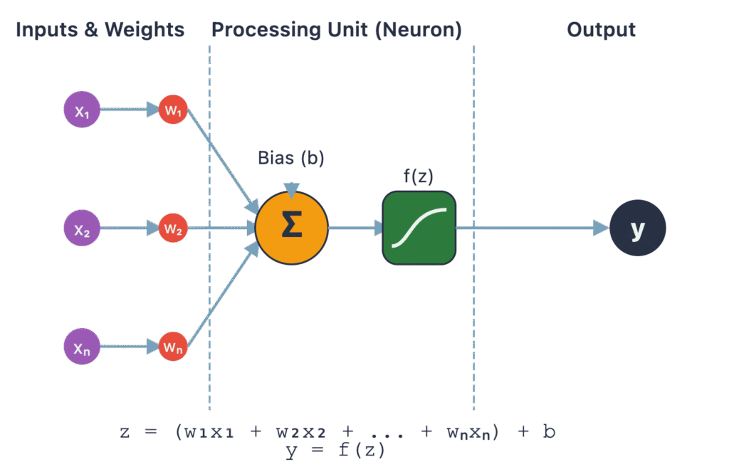
Comparison of Common Activation Functions
| Activation Function | Formula | Range | Pros | Cons |
|---|---|---|---|---|
| Sigmoid | 1 / (1 + e-x) | (0, 1) | Smooth gradient, output is probabilistic. Good for output layers in binary classification. | Vanishing gradient problem, output is not zero-centered, computationally expensive. |
| Tanh | (ex – e-x) / (ex + e-x) | (-1, 1) | Zero-centered output, which helps in optimization. | Still suffers from the vanishing gradient problem for large inputs. |
| ReLU | max(0, x) | [0, ∞) | Computationally efficient, avoids vanishing gradients for positive inputs, promotes sparsity. | “Dying ReLU” problem (neurons can become inactive), not zero-centered. |
| Leaky ReLU | max(0.01x, x) | (-∞, ∞) | Fixes the “Dying ReLU” problem by allowing a small, non-zero gradient for negative inputs. | Results are not always consistent; the optimal leakiness factor can vary. |
Autoencoders: Self-Supervised Neural Networks for Dimensionality Reduction
Shifting from topological methods, we enter the realm of deep learning with autoencoders. An autoencoder is a type of artificial neural network used to learn efficient data codings in an unsupervised (or, more accurately, self-supervised) manner. The fundamental idea is simple yet powerful: an autoencoder is trained to reconstruct its own input. It consists of two main parts: an encoder and a decoder. The encoder, \(f\), maps the high-dimensional input data \(\mathbf{x} \in \mathbb{R}^D\) to a low-dimensional latent space representation \(\mathbf{z} \in \mathbb{R}^d\), where \(d < D\). This latent vector \(\mathbf{z} = f(\mathbf{x})\) is the compressed representation of the input. The decoder, \(g\), then takes this latent vector and attempts to reconstruct the original input, producing \(\mathbf{x}’ = g(\mathbf{z})\).
The network is trained by minimizing a reconstruction loss function, \(L(\mathbf{x}, \mathbf{x}’)\), which measures the difference between the original input \(\mathbf{x}\) and the reconstructed output \(\mathbf{x}’\). Common loss functions include mean squared error (MSE) for continuous data or binary cross-entropy for binary data. The magic happens at the “bottleneck” layer—the latent space. Because the latent space has a smaller dimension than the input, the network is forced to learn the most salient features of the data to be able to reconstruct it accurately. It cannot simply memorize the input; it must learn a compressed representation that captures the core patterns and variations. This process effectively performs nonlinear dimensionality reduction. The encoder learns a complex, nonlinear mapping from the high-dimensional space to the low-dimensional manifold, and the decoder learns the reverse mapping. Once trained, the decoder is often discarded, and the encoder is used to transform new data into its low-dimensional latent representation for use in downstream tasks.
%%{ init: { 'flowchart': { 'curve': 'basis' } } }%%
graph TB
    subgraph Encoder
        direction LR
        Input(Input Data <b>x</b>) --> Enc1[Layer 1] --> Enc2[Layer 2] --> Enc3[Layer 3]
    end

    subgraph Bottleneck
        direction LR
        LatentSpace(Latent Space <b>z</b>)
    end

    subgraph Decoder
        direction LR
        Dec1[Layer 3] --> Dec2[Layer 2] --> Dec3[Layer 1] --> Output(Reconstructed Data <b>x'</b>)
    end

    Enc3 --> LatentSpace
    LatentSpace --> Dec1


    %% Styling
    classDef data fill:#9b59b6,stroke:#9b59b6,stroke-width:1px,color:#ebf5ee;
    classDef process fill:#78a1bb,stroke:#78a1bb,stroke-width:1px,color:#283044;
    classDef model fill:#e74c3c,stroke:#e74c3c,stroke-width:1px,color:#ebf5ee;
    classDef success fill:#2d7a3d,stroke:#2d7a3d,stroke-width:1px,color:#ebf5ee;

    class Input data;
    class Enc1,Enc2,Enc3,Dec1,Dec2,Dec3 process;
    class LatentSpace model;
    class Output success;
Variants of Autoencoders and Their Applications
The basic autoencoder architecture serves as a foundation for several powerful variants, each designed to address specific challenges and learn more robust representations.
- Denoising Autoencoders: To prevent the network from learning a trivial identity function (simply copying the input), denoising autoencoders are trained to reconstruct a clean input from a corrupted version. A stochastic corruption process (e.g., adding Gaussian noise, setting random inputs to zero) is applied to the input \(\mathbf{x}\) to get \(\tilde{\mathbf{x}}\). The network is then trained to minimize \(L(\mathbf{x}, g(f(\tilde{\mathbf{x}})))\). This forces the model to learn more robust features that are resilient to noise and capture the underlying data manifold rather than just the specific training examples.
- Sparse Autoencoders: Instead of imposing a bottleneck through dimensionality, sparse autoencoders have a latent space that can be larger than the input space. Sparsity is enforced by adding a regularization term to the loss function that penalizes the activations of the hidden layer neurons. This encourages the network to learn representations where only a small number of neurons are active at any given time for a given input. This leads to specialized neurons that learn to detect specific features, similar to how the human visual cortex is thought to operate.
- Variational Autoencoders (VAEs): VAEs are a more sophisticated, generative variant. Instead of mapping an input to a single point in the latent space, the encoder of a VAE maps it to a probability distribution, typically a multivariate Gaussian with a mean vector \(\boldsymbol{\mu}\) and a covariance matrix (usually diagonal, represented by a variance vector \(\boldsymbol{\sigma}^2\)). The latent vector \(\mathbf{z}\) is then sampled from this distribution. The loss function is composed of two terms: the standard reconstruction loss and a regularization term, the Kullback-Leibler (KL) divergence, which measures how much the learned distribution deviates from a standard normal distribution \(\mathcal{N}(0, \mathbf{I})\). This regularization forces the latent space to be continuous and well-structured, allowing for generation. By sampling points from the latent space and feeding them to the decoder, one can generate new, plausible data samples that resemble the training data. This makes VAEs powerful tools not just for dimensionality reduction but also for data augmentation and generative art.
%%{ init: { 'flowchart': { 'curve': 'basis' } } }%%
graph TD
    A(Input Data <b>x</b>) --> B[Encoder Network];

    subgraph Probabilistic Latent Space
        B --> C(Mean Vector <b>μ</b>);
        B --> D("Log-Variance Vector <b>log(σ<sup>2</sup>)</b>");
        E("Sample ε from N(0,I)");
        F("(<b>Reparameterization Trick</b><br>z = μ + ε * exp(0.5 * log(σ<sup>2</sup>)))")
    end

    C --> F;
    D --> F;
    E --> F;

    F --> G[Decoder Network];
    G --> H(Reconstructed Data <b>x'</b>);

    subgraph Two-Part Loss Function
        H -- 1. Reconstruction Loss --> I{"L(x, x')"};
        C -- 2. KL Divergence --> J{"KL( N(μ, σ<sup>2</sup>) || N(0,I) )"};
        D -- 2. KL Divergence --> J;
    end

    I --> K((Total Loss));
    J --> K;
    K -- Backpropagation --> B;
    K -- Backpropagation --> G;

    %% Styling
    classDef data fill:#9b59b6,stroke:#9b59b6,stroke-width:1px,color:#ebf5ee;
    classDef process fill:#78a1bb,stroke:#78a1bb,stroke-width:1px,color:#283044;
    classDef model fill:#e74c3c,stroke:#e74c3c,stroke-width:1px,color:#ebf5ee;
    classDef decision fill:#f39c12,stroke:#f39c12,stroke-width:1px,color:#283044;
    classDef success fill:#2d7a3d,stroke:#2d7a3d,stroke-width:1px,color:#ebf5ee;
    classDef warning fill:#f1c40f,stroke:#f1c40f,stroke-width:1px,color:#283044;

    class A,E data;
    class B,G,C,D process;
    class F,J,I,K warning;
    class H success;
These variants transform the autoencoder from a simple compression algorithm into a versatile tool for feature learning, anomaly detection (high reconstruction error can indicate an outlier), and generative modeling, making them a vital component of the modern AI engineering toolkit.
Practical Examples and Implementation
Development Environment Setup
To effectively implement the techniques discussed in this chapter, a modern Python environment with specific data science and deep learning libraries is required. We will primarily use scikit-learn for data handling, umap-learn for UMAP, and TensorFlow with its Keras API for building autoencoders. Matplotlib and Seaborn will be used for visualization.
Tip: It is highly recommended to use a virtual environment (e.g., using
venvorconda) to manage dependencies and avoid conflicts with other projects.
First, ensure you have Python 3.11 or newer installed. Then, install the necessary packages using pip:
# Create and activate a virtual environment (optional but recommended)
python -m venv ai_env
source ai_env/bin/activate  # On Windows, use `ai_env\Scripts\activate`

# Install the required libraries
pip install numpy pandas scikit-learn matplotlib seaborn
pip install umap-learn
pip install tensorflow
Library Versions :
numpy:1.26.xscikit-learn:1.4.xumap-learn:0.5.xtensorflow:2.16.x
This setup provides a robust foundation for both the topological approach of UMAP and the neural network-based approach of autoencoders. For the following examples, we will use the Fashion-MNIST dataset, a popular benchmark dataset consisting of 28×28 grayscale images of 10 different clothing items. It is slightly more complex than the classic MNIST dataset, making it a better test for these advanced techniques.
Core Implementation Examples
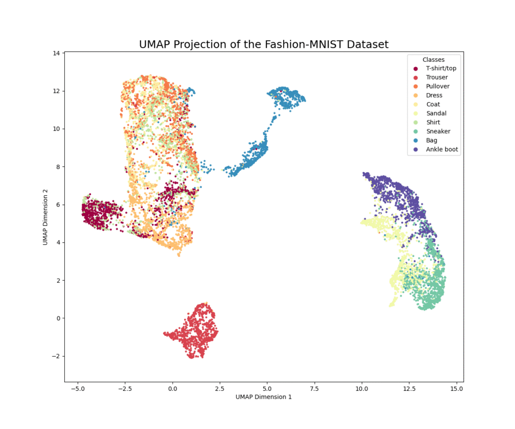
Example 1: Visualizing Fashion-MNIST with UMAP
This example demonstrates how to apply UMAP to the Fashion-MNIST dataset to create a 2D visualization. We will see how UMAP can effectively separate the different classes of clothing in the low-dimensional embedding.
import numpy as np
import umap
from tensorflow.keras.datasets import fashion_mnist
import matplotlib.pyplot as plt
import seaborn as sns

# Load the Fashion-MNIST dataset
(x_train, y_train), (x_test, y_test) = fashion_mnist.load_data()

# For performance, we'll use a subset of the data
# Using all 60,000 training images can be slow without a powerful machine
subset_size = 10000
indices = np.random.choice(x_train.shape[0], subset_size, replace=False)
x_subset = x_train[indices]
y_subset = y_train[indices]

# Reshape the data from 28x28 images to 784-dimensional vectors
x_flat = x_subset.reshape((subset_size, 28 * 28))

# Normalize the pixel values to be between 0 and 1
x_flat = x_flat.astype('float32') / 255.0

# Define the class names for plotting
class_names = ['T-shirt/top', 'Trouser', 'Pullover', 'Dress', 'Coat',
               'Sandal', 'Shirt', 'Sneaker', 'Bag', 'Ankle boot']

print("Data prepared. Starting UMAP embedding...")

# Initialize the UMAP reducer
# n_neighbors: Controls how UMAP balances local versus global structure.
# min_dist: Controls how tightly UMAP is allowed to pack points together.
# n_components: The dimension of the space to embed into.
reducer = umap.UMAP(n_neighbors=15, min_dist=0.1, n_components=2, random_state=42)

# Fit and transform the data
embedding = reducer.fit_transform(x_flat)

print("UMAP embedding complete. Plotting results...")

# Plot the results
plt.figure(figsize=(12, 10))
scatter = plt.scatter(embedding[:, 0], embedding[:, 1], c=y_subset, cmap='Spectral', s=5)
plt.gca().set_aspect('equal', 'datalim')
plt.title('UMAP Projection of the Fashion-MNIST Dataset', fontsize=18)
plt.xlabel('UMAP Dimension 1')
plt.ylabel('UMAP Dimension 2')

# Add a legend
plt.legend(handles=scatter.legend_elements()[0], labels=class_names, title="Classes")
plt.show()
Explanation:
The code first loads the Fashion-MNIST dataset and prepares a subset for efficiency. The images are flattened into 784-dimensional vectors and normalized. We then initialize the UMAP reducer with key hyperparameters: n_neighbors (a crucial parameter that determines the size of the local neighborhood the algorithm considers), min_dist (which controls the cosmetic appearance of the embedding), and n_components (set to 2 for visualization). The fit_transform method computes the low-dimensional embedding. The resulting plot should show distinct clusters corresponding to the different clothing categories, demonstrating UMAP’s ability to learn the underlying manifold of the image data. You’ll likely see that similar items, like “Sneaker” and “Ankle boot,” are located closer to each other than dissimilar items like “Trouser” and “Bag.”
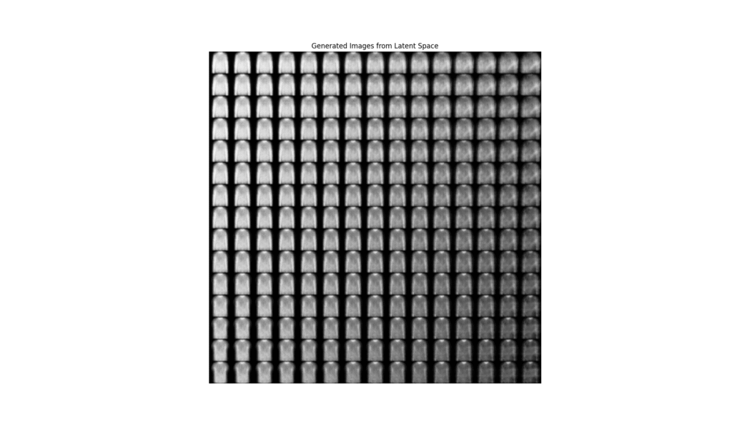
Example 2: Building a Variational Autoencoder (VAE) for Fashion-MNIST
This example implements a VAE to learn a compressed latent space for the Fashion-MNIST dataset. We will also demonstrate its generative capabilities by sampling from the latent space to create new clothing images.
import numpy as np
import tensorflow as tf
from tensorflow.keras import layers, models, backend as K
from tensorflow.keras.datasets import fashion_mnist
import matplotlib.pyplot as plt

# --- 1. Data Preparation ---
(x_train, y_train), (x_test, y_test) = fashion_mnist.load_data()
x_train = x_train.astype('float32') / 255.0
x_test = x_test.astype('float32') / 255.0
x_train = np.expand_dims(x_train, -1) # Add channel dimension
x_test = np.expand_dims(x_test, -1)

# --- 2. VAE Model Architecture ---
latent_dim = 2  # Dimensionality of the latent space
image_shape = (28, 28, 1)

# Sampling layer
class Sampling(layers.Layer):
    """Uses (z_mean, z_log_var) to sample z, the vector encoding a digit."""
    def call(self, inputs):
        z_mean, z_log_var = inputs
        batch = tf.shape(z_mean)[0]
        dim = tf.shape(z_mean)[1]
        epsilon = K.random_normal(shape=(batch, dim))
        return z_mean + tf.exp(0.5 * z_log_var) * epsilon

# --- Encoder ---
encoder_inputs = layers.Input(shape=image_shape)
x = layers.Conv2D(32, 3, activation='relu', strides=2, padding='same')(encoder_inputs)
x = layers.Conv2D(64, 3, activation='relu', strides=2, padding='same')(x)
x = layers.Flatten()(x)
x = layers.Dense(16, activation='relu')(x)
z_mean = layers.Dense(latent_dim, name='z_mean')(x)
z_log_var = layers.Dense(latent_dim, name='z_log_var')(x)
z = Sampling()([z_mean, z_log_var])
encoder = models.Model(encoder_inputs, [z_mean, z_log_var, z], name='encoder')
encoder.summary()

# --- Decoder ---
latent_inputs = layers.Input(shape=(latent_dim,))
x = layers.Dense(7 * 7 * 64, activation='relu')(latent_inputs)
x = layers.Reshape((7, 7, 64))(x)
x = layers.Conv2DTranspose(64, 3, activation='relu', strides=2, padding='same')(x)
x = layers.Conv2DTranspose(32, 3, activation='relu', strides=2, padding='same')(x)
decoder_outputs = layers.Conv2DTranspose(1, 3, activation='sigmoid', padding='same')(x)
decoder = models.Model(latent_inputs, decoder_outputs, name='decoder')
decoder.summary()

# --- VAE Model with Custom Loss ---
class VAE(models.Model):
    def __init__(self, encoder, decoder, **kwargs):
        super(VAE, self).__init__(**kwargs)
        self.encoder = encoder
        self.decoder = decoder
        self.total_loss_tracker = tf.keras.metrics.Mean(name="total_loss")
        self.reconstruction_loss_tracker = tf.keras.metrics.Mean(name="reconstruction_loss")
        self.kl_loss_tracker = tf.keras.metrics.Mean(name="kl_loss")

    @property
    def metrics(self):
        return [self.total_loss_tracker, self.reconstruction_loss_tracker, self.kl_loss_tracker]

    def train_step(self, data):
        with tf.GradientTape() as tape:
            z_mean, z_log_var, z = self.encoder(data)
            reconstruction = self.decoder(z)
            reconstruction_loss = tf.reduce_mean(
                tf.reduce_sum(
                    tf.keras.losses.binary_crossentropy(data, reconstruction), axis=(1, 2)
                )
            )
            kl_loss = -0.5 * (1 + z_log_var - tf.square(z_mean) - tf.exp(z_log_var))
            kl_loss = tf.reduce_mean(tf.reduce_sum(kl_loss, axis=1))
            total_loss = reconstruction_loss + kl_loss
        grads = tape.gradient(total_loss, self.trainable_weights)
        self.optimizer.apply_gradients(zip(grads, self.trainable_weights))
        self.total_loss_tracker.update_state(total_loss)
        self.reconstruction_loss_tracker.update_state(reconstruction_loss)
        self.kl_loss_tracker.update_state(kl_loss)
        return {m.name: m.result() for m in self.metrics}

# --- 3. Training ---
vae = VAE(encoder, decoder)
vae.compile(optimizer=tf.keras.optimizers.Adam())
vae.fit(x_train, epochs=30, batch_size=128)

# --- 4. Visualization and Generation ---
def plot_latent_space(vae, n=15, figsize=15):
    # display a n*n 2D manifold of digits
    digit_size = 28
    scale = 1.0
    figure = np.zeros((digit_size * n, digit_size * n))
    # linearly spaced coordinates corresponding to the 2D plot
    # of digit classes in the latent space
    grid_x = np.linspace(-scale, scale, n)
    grid_y = np.linspace(-scale, scale, n)[::-1]

    for i, yi in enumerate(grid_y):
        for j, xi in enumerate(grid_x):
            z_sample = np.array([[xi, yi]])
            x_decoded = vae.decoder.predict(z_sample, verbose=0)
            digit = x_decoded[0].reshape(digit_size, digit_size)
            figure[i * digit_size: (i + 1) * digit_size,
                   j * digit_size: (j + 1) * digit_size] = digit

    plt.figure(figsize=(figsize, figsize))
    plt.imshow(figure, cmap='Greys_r')
    plt.title("Generated Images from Latent Space")
    plt.axis('off')
    plt.show()

plot_latent_space(vae)
Explanation:
This code is more involved. It defines a convolutional VAE.
- Architecture: The encoder uses
Conv2Dlayers to downsample the image into a 16-dimensional vector, which is then mapped to thez_meanandz_log_varparameters of the latent distribution. The customSamplinglayer performs the reparameterization trick to samplez. The decoder usesConv2DTransposelayers to upsample the latent vector back into a 28×28 image. - Custom Loss: The VAE requires a custom loss function combining reconstruction loss (binary cross-entropy) and the KL divergence. We implement this within a custom
train_stepmethod by subclassingtf.keras.Model. - Training: The model is compiled and trained on the Fashion-MNIST data.
- Generation: The
plot_latent_spacefunction demonstrates the generative power of the VAE. It creates a grid over the 2D latent space, samples points from this grid, and passes them through the decoder to generate new images. The resulting plot shows a smooth transition between different types of clothing, highlighting the continuous and organized nature of the learned latent space.
Step-by-Step Tutorials
Tutorial: Interpreting UMAP Hyperparameters
Getting a good UMAP embedding often requires tuning its key hyperparameters. Let’s walk through the most important ones.
n_neighbors: This is arguably the most critical parameter. It controls the size of the local neighborhood UMAP considers for each point.- Low values (e.g., 2-5): UMAP will focus on very local structure. The resulting embedding will show fine-grained detail and may break up large clusters into smaller, intricate ones. This is useful for finding micro-clusters but can lose the global picture.
- High values (e.g., 50-200): UMAP will consider a larger neighborhood, forcing it to focus more on the global structure. The embedding will show broad relationships between clusters but may merge or obscure smaller, distinct groups.
- Default (15): This is a sensible default that often provides a good balance.
n_neighborsvalues (e.g., 5, 15, 50) to see how the structure of your data embedding changes.min_dist: This parameter controls the minimum distance between embedded points. It primarily affects the cosmetic appearance of the plot.- Low values (e.g., 0.0): Points will be packed very tightly together, resulting in dense, compact clusters. This is useful for emphasizing cluster separation.
- High values (e.g., 0.99): Points will be spread out more, resulting in a more uniform, fuzzy distribution. This is useful for seeing the broad topological structure of the data.
- Default (0.1): Provides a good balance between clustering and uniform distribution.
metric: This defines the distance metric used to measure similarity in the high-dimensional space.'euclidean'(default): Good for most dense, continuous data.'cosine': Excellent for high-dimensional, sparse data like text document vectors (TF-IDF) or gene expression data.'manhattan': Can be more robust to outliers than Euclidean.- Many others are available, including
'chebyshev','minkowski', etc. Choose the metric that best suits the nature of your data.
By systematically adjusting these parameters, you can tailor the UMAP embedding to best reveal the structures of interest in your specific dataset.
Industry Applications and Case Studies
- Genomics and Single-Cell RNA Sequencing (scRNA-seq): In bioinformatics, scRNA-seq data is notoriously high-dimensional, with measurements for thousands of genes across tens of thousands of cells. UMAP has become the de facto standard for visualizing this data. It allows researchers to project cells into a 2D or 3D space where cells with similar gene expression profiles cluster together. This is crucial for identifying different cell types, discovering new cell subtypes, and understanding developmental trajectories in tissues. The ability of UMAP to preserve both local and global structure helps reveal the complex relationships between cell populations, accelerating research in cancer, immunology, and developmental biology.
- Anomaly Detection in Cybersecurity: Autoencoders are widely used for unsupervised anomaly detection in network traffic and system logs. A standard autoencoder is trained exclusively on “normal” data (e.g., network packets from benign traffic). The model learns to reconstruct this normal data with very low error. When the trained model is presented with anomalous data (e.g., a packet from a malware attack), it fails to reconstruct it accurately, resulting in a high reconstruction error. By setting a threshold on this error, security systems can flag potential threats in real-time. Denoising autoencoders are particularly effective here as they learn more robust representations of normality, making them less susceptible to minor, benign variations in the data.
- Feature Engineering for Recommender Systems: In e-commerce and content streaming, user-item interaction matrices are often massive and sparse. Autoencoders can be used to learn dense, low-dimensional latent representations (embeddings) for both users and items. For example, an autoencoder can be trained to reconstruct a user’s interaction vector (e.g., a vector of movie ratings). The activations of the bottleneck layer then serve as a rich, compressed feature vector for that user. These learned embeddings capture complex, nonlinear relationships in user preferences and can be fed into downstream models (like collaborative filtering or gradient boosted trees) to generate more accurate and personalized recommendations, significantly improving user engagement and business value.
Best Practices and Common Pitfalls
- Don’t Interpret Cluster Distances in UMAP Literally: While UMAP is excellent at preserving the topological structure of data, the relative distances between well-separated clusters in the final embedding are not always meaningful. UMAP’s optimization process focuses on preserving local neighborhood graphs, and the global arrangement is a secondary effect. A large gap between two clusters does not necessarily mean they are “more different” than two clusters with a smaller gap. Focus on the clustering, the relative positions of points within clusters, and the connections between them, rather than the absolute distances in the 2D plane.
- Autoencoder Architecture Matters: The design of your autoencoder’s encoder and decoder networks is critical. A network that is too simple (too few layers or neurons) may underfit, failing to capture the complexity of the data manifold and leading to poor reconstructions. Conversely, a network that is too powerful, especially one with a large bottleneck layer, may overfit by learning a trivial identity function that simply passes the data through without learning a meaningful compressed representation. Start with a simple, symmetric architecture and gradually increase complexity. Use techniques like dropout and weight decay to prevent overfitting.
- The Curse of the “Hairball”: A common failure mode for UMAP (and t-SNE) is producing a dense, uninterpretable “hairball” where all points are clumped together. This often happens when the
n_neighborsparameter is set too high for the dataset size, or when the data lacks any discernible structure. If you see this, try significantly reducingn_neighborsto focus on more local patterns. Also, ensure your data is properly scaled and preprocessed, as features with large variances can dominate the distance calculations. - VAE Training Instability: Training Variational Autoencoders can be challenging. The balance between the reconstruction loss and the KL divergence term is delicate. If the KL term’s weight is too high, the model may prioritize matching the prior \(\mathcal{N}(0, \mathbf{I})\) at the expense of reconstruction quality, leading to a phenomenon known as “posterior collapse” where the encoder ignores the input. If it’s too low, the latent space may lose its regularized, continuous structure. Techniques like KL annealing (gradually increasing the weight of the KL term during training) can help stabilize the process and achieve a better balance.
- Scalability and Productionization: While UMAP is significantly faster than t-SNE, for truly massive datasets (millions of points), fitting can still be time-consuming. UMAP’s
transformmethod allows you to embed new data points into an existing embedding, which is crucial for production systems where you can’t refit the model for every new data point. For autoencoders, once the model is trained, the encoder part is typically a lightweight neural network that can perform inference very quickly, making it well-suited for real-time feature extraction in production environments.
Hands-on Exercises
- Basic: UMAP Hyperparameter Tuning:
- Objective: Understand the impact of
n_neighborsandmin_diston the UMAP embedding. - Task: Using the UMAP implementation from the chapter on the full Fashion-MNIST training set (60,000 images), generate four different plots:
- Low
n_neighbors(e.g., 5), lowmin_dist(e.g., 0.01) - Low
n_neighbors(e.g., 5), highmin_dist(e.g., 0.8) - High
n_neighbors(e.g., 100), lowmin_dist(e.g., 0.01) - High
n_neighbors(e.g., 100), highmin_dist(e.g., 0.8)
- Low
- Expected Outcome: A report (e.g., a Jupyter Notebook with markdown) describing how each parameter combination affects the visualization. Which setting is best for separating classes? Which is best for seeing the overall structure?
- Objective: Understand the impact of
- Intermediate: Denoising Autoencoder for Image Restoration:
- Objective: Implement a denoising autoencoder to remove noise from images.
- Task:
- Take the Fashion-MNIST dataset.
- Create a noisy version of the dataset by adding random Gaussian noise to each image (
x_train_noisy = x_train + 0.5 * np.random.normal(...)). Remember to clip the values to stay between 0 and 1. - Build a convolutional autoencoder (similar to the VAE structure but without the sampling layer and KL loss).
- Train the autoencoder to take the noisy images as input and reconstruct the original, clean images.
- Expected Outcome: A script that trains the model and a visualization showing a few examples of the original image, the noisy image, and the autoencoder’s reconstructed (denoised) image.
- Advanced: Dimensionality Reduction for Downstream Classification:
- Objective: Compare the effectiveness of UMAP and a VAE as feature engineering tools for a classification task.
- Task:
- Use the Fashion-MNIST dataset.
- Path A (UMAP): Train a UMAP reducer on
x_trainto reduce the dimensionality to a reasonable number (e.g., 32). Use this reducer to transform bothx_trainandx_test. - Path B (VAE): Train the VAE from the chapter on
x_train. Use the trained encoder to transformx_trainandx_testinto their latent representations (z_mean). - Benchmark: Train a simple classifier (e.g.,
LogisticRegressionor a smallRandomForestfromscikit-learn) on three versions of the data: (a) the original flattened images, (b) the UMAP-transformed features, and (c) the VAE-encoded features.
- Expected Outcome: A comparison of the classification accuracy for all three feature sets. Which dimensionality reduction technique produced more useful features for the classifier? Discuss why you think one performed better than the other.
Tools and Technologies
umap-learn: The primary Python library for UMAP. It is highly optimized, built onnumbafor high performance, and integrates well with thescikit-learnAPI (fit,transform). It is the go-to tool for applying UMAP in practice.TensorFlow/Keras: A leading deep learning framework used for building and training autoencoders. Its high-level Keras API makes it easy to define complex neural network architectures, custom layers, and training loops, as demonstrated in the VAE example.PyTorch: An alternative, equally powerful deep learning framework. It is known for its flexibility and more “Pythonic” feel, and is also an excellent choice for implementing autoencoder models.scikit-learn: A fundamental library in the Python data science ecosystem. While it doesn’t contain implementations of UMAP or advanced autoencoders, it is essential for data preprocessing (StandardScaler), model evaluation (accuracy_score), and training baseline models for comparison.Matplotlib&Seaborn: The standard libraries for data visualization in Python. They are crucial for plotting the low-dimensional embeddings produced by UMAP and autoencoders and for visualizing the generative results of VAEs.
Summary
- Manifold Hypothesis: High-dimensional data often lies on a lower-dimensional, nonlinear manifold. Advanced dimensionality reduction techniques aim to uncover this underlying structure.
- UMAP: A powerful manifold learning technique based on topological data analysis. It excels at preserving both local and global data structure, is computationally efficient, and is highly effective for visualization and feature engineering. Its key hyperparameters are
n_neighborsandmin_dist. - Autoencoders: A family of self-supervised neural networks that learn compressed data representations by reconstructing their input. The bottleneck layer forces the network to learn a meaningful, low-dimensional latent space.
- Autoencoder Variants: Denoising autoencoders learn robust features by reconstructing clean data from corrupted inputs. Variational Autoencoders (VAEs) learn a continuous, probabilistic latent space, enabling them to function as generative models.
- Practical Implementation: UMAP can be easily implemented with the
umap-learnlibrary, while autoencoders are built using deep learning frameworks likeTensorFloworPyTorch. - Applications: These techniques are critical in fields like genomics for cell type identification, cybersecurity for anomaly detection, and e-commerce for building powerful recommender systems.
- Best Practices: It is crucial to tune hyperparameters thoughtfully, understand the limitations of each method (e.g., interpreting UMAP cluster distances), and choose the right tool for the task at hand.
High-Level Algorithm Comparison for AI Engineering
| Algorithm | Problem Type | Strengths | Weaknesses | Best Use Cases |
|---|---|---|---|---|
| UMAP | Dimensionality Reduction, Visualization |
Excellent at preserving both local and global data structure.
Computationally efficient and scalable.
Flexible distance metric options.
|
Output is stochastic; results can vary between runs.
Inter-cluster distances are not always meaningful.
|
Visualizing high-dimensional data (e.g., genomics, embeddings), scalable manifold learning, feature engineering. |
| Autoencoder | Dimensionality Reduction, Feature Learning, Anomaly Detection |
Learns complex, non-linear data representations.
Can be tailored (denoising, sparse) for robust feature extraction.
The encoder can be used for fast inference on new data.
|
Requires careful architecture design to avoid overfitting.
Latent space may not be continuous or well-structured.
|
Image compression/denoising, learning embeddings for recommender systems, unsupervised anomaly detection. |
| Variational Autoencoder (VAE) | Generative Modeling, Dimensionality Reduction |
Generates new, plausible data samples.
Learns a continuous, structured latent space suitable for interpolation.
|
Training can be unstable and sensitive to hyperparameters.
Generated samples can be blurrier than those from GANs.
|
Data augmentation, generative art, learning smooth representations of data for tasks like drug discovery. |
| Principal Component Analysis (PCA) | Dimensionality Reduction |
Deterministic and fast.
Provides an orthogonal, interpretable basis (principal components).
|
Only captures linear relationships in the data.
Can fail on data with complex, non-linear manifold structures.
|
A fast baseline for dimensionality reduction, data whitening, noise reduction in linear systems. |
Further Reading and Resources
- UMAP: Uniform Manifold Approximation and Projection for Dimension Reduction (McInnes, L., Healy, J., & Melville, J., 2018): The original research paper introducing UMAP. A must-read for a deep theoretical understanding. Available on arXiv. https://arxiv.org/abs/1802.03426
- Official
umap-learnDocumentation: The most comprehensive and up-to-date resource for using the UMAP library, including detailed API references, tutorials, and advanced usage examples. https://umap-learn.readthedocs.io/en/latest/ - “An Introduction to Variational Autoencoders” (Kingma, D. P., & Welling, M.): A foundational tutorial on VAEs from the original authors. Provides an intuitive yet mathematically rigorous explanation.
- Deep Learning with Python, Second Edition (by François Chollet): An excellent book that provides practical, hands-on introductions to building neural networks, including autoencoders, with Keras and TensorFlow.
- Distill.pub: An online journal with outstanding articles that visually and interactively explain complex machine learning concepts. Their articles on dimensionality reduction and generative models are particularly insightful.
- “How to Use t-SNE Effectively” (Wattenberg, et al., Distill.pub): While focused on t-SNE, this article provides invaluable intuition about how manifold learning algorithms work and how to interpret their outputs, much of which is directly applicable to UMAP.
- TensorFlow Tutorials – Variational Autoencoder: The official TensorFlow website includes a detailed, end-to-end tutorial on building and training a VAE, which serves as an excellent practical guide.
Glossary of Terms
- Autoencoder: A type of neural network composed of an encoder and a decoder, trained to reconstruct its input. It is used for unsupervised dimensionality reduction and feature learning.
- Curse of Dimensionality: A term describing the various phenomena that arise when analyzing and organizing data in high-dimensional spaces that do not occur in low-dimensional settings.
- Decoder: The part of an autoencoder that reconstructs the original data from its latent space representation.
- Encoder: The part of an autoencoder that maps the input data to a lower-dimensional latent space representation.
- Kullback-Leibler (KL) Divergence: A measure of how one probability distribution is different from a second, reference probability distribution. In VAEs, it is used to regularize the latent space.
- Latent Space: The low-dimensional space where the compressed representation of the data (the “encoding”) resides.
- Manifold: A topological space that locally resembles Euclidean space near each point. In ML, it refers to the lower-dimensional surface on which high-dimensional data is assumed to lie.
- Manifold Hypothesis: The assumption that real-world high-dimensional data is concentrated near a low-dimensional, nonlinear manifold.
- Reconstruction Loss: The loss function used to train an autoencoder, which measures the difference between the original input and the reconstructed output.
- Simplicial Complex: A topological space constructed by “gluing together” points, line segments, triangles, and their n-dimensional counterparts. UMAP uses a “fuzzy” version of this concept.
- Uniform Manifold Approximation and Projection (UMAP): An advanced dimensionality reduction technique based on manifold learning and topological data analysis, known for its speed and ability to preserve both local and global data structure.
- Variational Autoencoder (VAE): A generative type of autoencoder that learns a probabilistic latent space, allowing for the generation of new data samples.
