
Chapter 18: Advanced Data Structures and Algorithms for AI Engineering
Chapter Objectives
Upon completing this chapter, students will be able to:
- Analyze the time and space complexity of algorithms using Big O notation to select the most efficient solutions for data-intensive AI tasks.
- Implement advanced data structures such as deques, heaps, and graphs from scratch and apply them to solve common problems in machine learning, such as pathfinding and feature management.
- Design and develop robust, scalable AI applications by applying Object-Oriented Programming (OOP) principles to model complex systems and relationships.
- Leverage functional programming paradigms to build clean, predictable, and parallelizable data processing pipelines for machine learning workflows.
- Optimize Python code for performance-critical AI applications by profiling and selecting appropriate data structures and algorithms for specific computational challenges.
- Translate theoretical algorithmic concepts into practical, efficient Python code using standard libraries like
collections,heapq, anditertoolsto build foundational components of AI systems.
Introduction
In the landscape of modern Artificial Intelligence, Python is not merely a language but the lingua franca—the foundational medium through which abstract theories are transformed into tangible, world-changing technologies. While introductory programming skills can power simple scripts, the construction of sophisticated, production-grade AI systems demands a far deeper level of mastery. This chapter bridges the gap between basic competency and professional expertise, delving into the advanced data structures, algorithmic principles, and programming paradigms that underpin high-performance AI engineering. We will explore why the choice between a list and a deque can mean the difference between a sluggish prototype and a real-time analytics engine, or how object-oriented design principles enable the creation of modular and extensible machine learning frameworks like TensorFlow and PyTorch.
This chapter moves beyond syntax to embrace the “Pythonic” philosophy of clarity, simplicity, and readability, principles that are paramount when building complex systems that must be maintained, scaled, and collaborated on by teams of engineers. We will investigate how to analyze algorithmic efficiency with Big O notation, a critical skill for handling the massive datasets common in AI. We will then connect these theoretical underpinnings to the practical tools of the trade, implementing data structures that form the backbone of everything from recommendation engines to natural language processing models. By the end of this chapter, you will not just write Python code; you will wield it with the precision and foresight of a seasoned AI engineer, ready to build the next generation of intelligent systems.
Technical Background
The Pythonic Mindset for AI Engineering
At the heart of effective Python programming lies a philosophy often referred to as “The Zen of Python.” This collection of 20 aphorisms, accessible by typing import this into a Python interpreter, emphasizes principles like “Beautiful is better than ugly,” “Explicit is better than implicit,” and “Readability counts.” For an AI engineer, these are not mere suggestions but core tenets for building sustainable and robust systems. AI code is rarely a one-off script; it is a living asset that undergoes constant iteration, debugging, and extension. A model’s training pipeline, a data preprocessing script, or an inference API must be understood by multiple team members over a long lifecycle. When code is readable and explicit, it becomes easier to debug, maintain, and optimize. For instance, a complex feature engineering pipeline written with clear variable names and a logical flow is far less prone to subtle, data-corrupting bugs than a dense, uncommented block of code. This philosophy directly impacts collaboration and project velocity, making it a pragmatic, business-critical concern.
The Pythonic approach also favors simplicity. In AI, where models can already be black boxes, the surrounding code should be as transparent as possible. Instead of writing overly clever “one-liners” that are difficult to parse, a Pythonic developer will often choose a more verbose but clearer multi-line equivalent. This is particularly important in debugging, where tracing the flow of data through a complex series of transformations is a common task. Furthermore, the principle of “There should be one—and preferably only one—obvious way to do it” guides developers toward using standard libraries and established patterns. This consistency across a codebase and the broader Python ecosystem means that engineers can more quickly understand and contribute to new projects. Adopting this mindset is the first step toward writing professional-grade AI code that is not just functional but also scalable, maintainable, and a pleasure to work with.
Advanced Data Structures in Action
Beyond Lists and Dictionaries: Specialized Collections
While Python’s built-in list and dict types are powerful general-purpose containers, high-performance AI applications often require more specialized data structures to handle specific operational patterns efficiently. The collections module provides several high-performance container datatypes that serve as “batteries-included” solutions for these scenarios. One of the most valuable is the deque (double-ended queue). A deque is implemented as a doubly-linked list, which provides highly efficient appends and pops from both the left and right ends. While appending to a standard list is an amortized \(O(1)\) operation, prepending or popping from the left (list.pop(0)) is an \(O(n)\) operation because all subsequent elements must be shifted. In contrast, for a deque, both appendleft() and popleft() are \(O(1)\) operations. This makes deque the ideal choice for implementing sliding windows over sequential data, such as in time-series analysis or for processing tokens in a natural language processing pipeline.
Another essential tool is the defaultdict, a subclass of dict that provides a default value for a nonexistent key. This elegantly avoids the need for cumbersome if key in dict checks. For example, when building a vocabulary from a text corpus, a defaultdict(int) can be used to count word frequencies; if a word is encountered for the first time, its key is automatically initialized with int(), which is 0, before the increment operation proceeds. Similarly, collections.Counter is a specialized dictionary designed for counting hashable objects, providing a streamlined way to implement techniques like Bag-of-Words in NLP or to analyze the distribution of classes in a dataset. For tasks requiring a priority queue, such as in pathfinding algorithms like A* or for managing events in a simulation, Python’s heapq module provides an efficient min-heap implementation. Unlike a sorted list, where insertion is \(O(n)\), adding an item to a heap is an \(O(\log n)\) operation, making it vastly more performant for dynamic ordering tasks. Understanding the performance characteristics and use cases of these specialized structures is crucial for writing optimized AI code.
Python Data Structure Performance (Time Complexity)
| Operation | list | collections.deque | heapq (min-heap) | Notes |
|---|---|---|---|---|
| Append (to end) | O(1) | O(1) | O(log n) | List append is amortized O(1). Heap push is O(log n). |
| Prepend (to start) | O(n) | O(1) | N/A | This is the key advantage of a deque over a list. |
| Pop (from end) | O(1) | O(1) | N/A | Heaps do not support arbitrary pops efficiently. |
| Pop (from start) | O(n) | O(1) | O(log n) | Popping from a heap always removes the smallest element. |
| Get Item (by index) | O(1) | O(n) | O(n) | Only lists provide fast random access. Deque access is O(n) from the ends. |
| Get Smallest Item | O(n) | O(n) | O(1) | Accessing the smallest item is the primary use case for a min-heap. |
Trees and Graphs: The Backbone of Complex Models
Many systems and problems in AI are fundamentally about relationships and hierarchical structures, which are naturally modeled by trees and graphs. A tree is a hierarchical data structure consisting of nodes connected by edges, with a single root node and no cycles. A graph is a more general structure of nodes (vertices) and edges, which can contain cycles and multiple connected components. In Python, these are typically implemented using classes for nodes and an adjacency list (often a dictionary mapping a node to a list of its neighbors) to represent the connections. This representation is memory-efficient for sparse graphs, which are common in real-world applications.
These abstract structures have concrete applications across AI. A classic decision tree algorithm, for instance, builds a tree where each internal node represents a test on a feature, each branch represents the outcome of the test, and each leaf node represents a class label. Traversing the tree from the root down to a leaf provides the prediction. Neural networks themselves can be conceptualized as complex, layered graphs where nodes are neurons and edges are the weighted connections between them. The process of forward and backward propagation involves traversing this computation graph. Beyond models, graphs are essential for representing knowledge. A knowledge graph can capture relationships between entities (e.g., “Paris” -[is capital of]-> “France”), forming the basis for advanced search engines and question-answering systems. Understanding how to traverse these structures is equally critical. Depth-First Search (DFS) and Breadth-First Search (BFS) are fundamental traversal algorithms. BFS, which explores neighbor nodes first, is used in algorithms like shortest path finding on unweighted graphs, while DFS, which explores as far as possible along each branch, is useful for tasks like topological sorting or detecting cycles.
Algorithmic Efficiency and Complexity
Big O Notation in Practice
In the domain of AI, where datasets can contain billions of data points, the efficiency of an algorithm is not an academic concern—it is a critical factor determining a project’s feasibility. Big O notation is the language we use to describe the performance or complexity of an algorithm as the input size, \(n\), grows. It provides an upper bound on the growth rate of the function, allowing us to abstract away from the specifics of hardware and focus on the inherent scalability of the approach. For an AI engineer, a practical understanding of Big O is essential for making informed decisions. For example, an algorithm with a time complexity of \(O(n^2)\) (quadratic time) might be perfectly acceptable for a dataset with 1,000 samples, but it would be computationally intractable for a dataset with 1 million samples.
Common complexity classes seen in AI include \(O(1)\) (constant time), where the execution time is independent of the input size, such as accessing an element in a dictionary by its key. An algorithm with \(O(\log n)\) complexity (logarithmic time), like binary search, is extremely efficient, as the time required grows very slowly with \(n\). Data preprocessing steps that iterate through a dataset once, such as normalizing features, typically have \(O(n)\) complexity (linear time). More advanced algorithms, like efficient sorting algorithms (e.g., Merge Sort), have \(O(n \log n)\) complexity. The dreaded \(O(n^2)\) and \(O(2^n)\) (exponential time) complexities often arise from naive implementations, such as nested loops that compare every element in a dataset to every other element. When designing a feature engineering pipeline or selecting a machine learning algorithm, analyzing the Big O complexity of each step allows an engineer to identify potential bottlenecks and choose a more scalable approach, saving invaluable computational resources and development time.

Sorting and Searching for AI Applications
Sorting and searching are foundational algorithmic problems that appear in various guises within AI workflows. While Python’s built-in sort() method is highly optimized (using an algorithm called Timsort, which has a worst-case complexity of \(O(n \log n)\)), understanding the principles behind different sorting algorithms provides deeper insight into computational trade-offs. Merge Sort, for example, is a classic divide-and-conquer algorithm that recursively splits the input array in half, sorts the subarrays, and then merges them back together. Its guaranteed \(O(n \log n)\) performance makes it very reliable. Quick Sort also uses a divide-and-conquer strategy but works by partitioning the array around a pivot element. While its average-case performance is also \(O(n \log n)\) and it is often faster in practice due to lower constant factors and being an in-place sort (less memory usage), its worst-case performance is \(O(n^2)\), a risk that must be considered.
Searching is equally critical. When dealing with large, sorted datasets—such as a sorted list of feature IDs or a timeline of events—binary search is the go-to algorithm. It works by repeatedly dividing the search interval in half, achieving an exceptionally efficient \(O(\log n)\) time complexity. This is exponentially faster than a linear search (\(O(n)\)). In AI, this can be applied to tasks like finding the optimal threshold in a decision tree or efficiently searching through a sorted hyperparameter space during model tuning. More complex search problems, such as finding the best sequence of actions in a reinforcement learning environment or finding the shortest path in a graph, require more advanced algorithms like Dijkstra’s or A*, which build upon these fundamental searching and data structure principles. These algorithms intelligently explore a search space, using priority queues (often implemented with heaps) to efficiently decide which path to explore next, demonstrating the deep interplay between data structures and algorithms.
Comparison of Common Machine Learning Algorithms
| Algorithm | Problem Type | Strengths | Weaknesses | Best Use Cases |
|---|---|---|---|---|
| Linear Regression | Regression | Simple, interpretable, fast to train. No hyperparameters. | Assumes linear relationship. Sensitive to outliers. | Baseline models, predicting continuous values (e.g., house prices, sales). |
| Logistic Regression | Classification | Interpretable, efficient, provides probabilities. Good for binary classification. | Assumes linearity between features and log-odds. | Spam detection, medical diagnosis, credit scoring. |
| Decision Tree | Classification, Regression | Easy to visualize and understand. Handles non-linear data. | Prone to overfitting. Can be unstable. | Customer segmentation, feature importance analysis, simple rule-based systems. |
| Random Forest | Classification, Regression | High accuracy. Robust to overfitting. Handles missing values. | Less interpretable than a single tree. Can be slow to train on large datasets. | Fraud detection, stock market prediction, image classification. |
| Support Vector Machine (SVM) | Classification, Regression | Effective in high-dimensional spaces. Memory efficient. | Doesn’t perform well on large datasets. Less effective on noisy data. | Text classification, face detection, bioinformatics. |
| K-Nearest Neighbors (KNN) | Classification, Regression | Simple to implement. No training phase (lazy learner). | Computationally expensive during prediction. Sensitive to irrelevant features. | Recommendation systems, image recognition, anomaly detection. |
| K-Means | Clustering | Simple and fast for large datasets. Easy to implement. | Must specify number of clusters (K). Sensitive to initial centroids. | Market segmentation, document clustering, image compression. |
| Neural Network | Classification, Regression, etc. | Can model highly complex, non-linear relationships. State-of-the-art performance. | Requires large amounts of data. Computationally intensive. “Black box” nature. | Image recognition, natural language processing, autonomous driving. |
Programming Paradigms for Scalable AI
Object-Oriented Programming for Model Design
Object-Oriented Programming (OOP) is a paradigm that structures a program by bundling related properties and behaviors into individual “objects.” For AI engineering, OOP is not just a way to organize code; it’s a powerful methodology for modeling the complex components of an AI system in a way that is modular, reusable, and extensible. The core principles of OOP—encapsulation, inheritance, and polymorphism—find direct application in the design of machine learning frameworks and applications.
Encapsulation refers to the bundling of data (attributes) and the methods that operate on that data into a single unit, or class. This is fundamental to creating a clean model API. For example, a NeuralNetwork class would encapsulate its layers, weights, and biases, along with methods like forward() for prediction and backward() for training. This prevents direct, uncontrolled access to the model’s internal state, reducing complexity and preventing bugs. Inheritance allows a new class (subclass) to inherit attributes and methods from an existing class (superclass). This is extensively used in ML frameworks to create a hierarchy of models or layers. One might define a base Layer class with common functionality, and then create specific DenseLayer, ConvolutionalLayer, and RecurrentLayer subclasses that inherit from it and implement their unique forward and backward passes. This promotes code reuse and establishes a common interface. Polymorphism (literally “many forms”) allows objects of different classes to be treated as objects of a common superclass. This means you can write generic code that operates on objects of the base class, and it will work correctly for any subclass. For instance, a training loop can iterate through a list of Layer objects and call a forward() method on each one, regardless of its specific type, making the entire system incredibly flexible and easy to extend with new layer types.
erDiagram
    Layer {
        string name
        shape input_shape
        shape output_shape
        method forward
        method backward
    }

    DenseLayer {
        matrix weights
        vector biases
        method forward
        method backward
    }

    ConvolutionalLayer {
        tensor filters
        tuple kernel_size
        method forward
        method backward
    }

    Model {
        list layers
        method add
        method predict
        method train
    }

    TrainingData {
        tensor data
        tensor labels
        int batch_size
    }

    Weights {
        matrix weight_matrix
        vector bias_vector
        float learning_rate
    }

    Gradient {
        tensor gradient_values
        string layer_name
        int step
    }

    %% Inheritance relationships
    Layer ||--o{ DenseLayer : "IS-A"
    Layer ||--o{ ConvolutionalLayer : "IS-A"

    %% Composition relationships
    Model ||--o{ Layer : "CONTAINS"
    Model ||--o{ DenseLayer : "HAS"
    Model ||--o{ ConvolutionalLayer : "HAS"

    %% Training relationships
    Model ||--o{ TrainingData : "TRAINS-ON"
    DenseLayer ||--o{ Weights : "OWNS"
    ConvolutionalLayer ||--o{ Weights : "OWNS"

    %% Backpropagation relationships
    Layer ||--o{ Gradient : "PRODUCES"
    DenseLayer ||--o{ Gradient : "COMPUTES"
    ConvolutionalLayer ||--o{ Gradient : "COMPUTES"
Functional Programming for Data Pipelines
While OOP excels at modeling stateful objects like models, Functional Programming (FP) offers a complementary paradigm that is exceptionally well-suited for the stateless, transformational nature of data processing pipelines. The core idea of FP is to treat computation as the evaluation of mathematical functions and to avoid changing state and mutable data. Key concepts include pure functions, immutability, and the use of higher-order functions. A pure function is one whose output value is determined only by its input values, with no observable side effects. This makes them easy to reason about, test, and debug. When a data transformation function is pure, you can be certain it won’t unexpectedly modify data elsewhere in the system.
Immutability, the principle that data cannot be changed after it’s created, is another cornerstone. Instead of modifying a data structure in-place, a functional approach creates a new data structure with the updated values. This prevents a whole class of bugs related to shared mutable state, which is especially important in concurrent or distributed computing environments common in big data processing with tools like Spark. Python supports functional programming through features like lambda functions and built-in higher-order functions such as map(), filter(), and reduce(). The map() function applies a function to every item of an iterable, filter() creates an iterator from elements of an iterable for which a function returns true, and functools.reduce() applies a function of two arguments cumulatively to the items of a sequence. By chaining these operations, one can build elegant, declarative, and highly readable data preprocessing pipelines. For example, a pipeline to clean and tokenize text data can be expressed as a series of small, pure, and testable functions, making the entire workflow more robust and maintainable.
        graph TD
            A[Raw Data<br><i>e.g., list of text documents</i>] --> B(<b>map</b>: clean_text_function);
            B --> C(<b>map</b>: tokenize_function);
            C --> D(<b>filter</b>: remove_stopwords_function);
            D --> E(<b>map</b>: stem_words_function);
            E --> F[Processed Data<br><i>e.g., list of token lists</i>];

            %% Styling
            style A fill:#9b59b6,stroke:#9b59b6,stroke-width:1px,color:#ebf5ee
            style B fill:#78a1bb,stroke:#78a1bb,stroke-width:1px,color:#283044
            style C fill:#78a1bb,stroke:#78a1bb,stroke-width:1px,color:#283044
            style D fill:#f39c12,stroke:#f39c12,stroke-width:1px,color:#283044
            style E fill:#78a1bb,stroke:#78a1bb,stroke-width:1px,color:#283044
            style F fill:#2d7a3d,stroke:#2d7a3d,stroke-width:2px,color:#ebf5ee

            linkStyle 0 stroke:#78a1bb,stroke-width:2px;
            linkStyle 1 stroke:#78a1bb,stroke-width:2px;
            linkStyle 2 stroke:#78a1bb,stroke-width:2px;
            linkStyle 3 stroke:#78a1bb,stroke-width:2px;
Practical Examples and Implementation
Mathematical Concept Implementation
Many advanced data structures are direct implementations of mathematical concepts. A graph, for instance, is a representation of a set of objects where some pairs of objects are connected. In Python, we can implement this concept using classes and dictionaries to create a flexible and efficient structure. The Node or Vertex can be a simple class, while the Graph itself manages the connections, often through an adjacency list. This allows us to translate the abstract theory of graph algorithms into concrete, executable code.
Here is a practical implementation of a directed graph in Python, which can be used to model everything from social networks to the flow of computation in a neural network.
# A complete, working example of a directed graph implementation
import collections

class Graph:
    """
    A class to represent a directed graph using an adjacency list.
    The adjacency list is implemented as a dictionary where keys are node identifiers
    and values are lists of identifiers of their neighbors.
    """
    def __init__(self):
        # The adjacency list is stored in a defaultdict to simplify adding new nodes.
        # When a node is first accessed, it will be automatically added with an empty list.
        self.adj_list = collections.defaultdict(list)

    def add_edge(self, u, v):
        """
        Adds a directed edge from node u to node v.
        """
        # Appending v to the list of u's neighbors establishes the connection.
        self.adj_list[u].append(v)
        # Ensure node v is also in the graph, even if it has no outgoing edges.
        if v not in self.adj_list:
            self.adj_list[v] = []

    def __str__(self):
        """
        Provides a string representation of the graph for easy printing.
        """
        return str(dict(self.adj_list))

    def bfs(self, start_node):
        """
        Performs a Breadth-First Search (BFS) starting from a given node.
        Returns the list of visited nodes in the order they were visited.
        BFS is useful for finding the shortest path in an unweighted graph.
        """
        if start_node not in self.adj_list:
            print(f"Error: Start node {start_node} not in graph.")
            return []

        visited = set()
        queue = collections.deque([start_node])
        visited.add(start_node)
        traversal_order = []

        while queue:
            # Dequeue a vertex from the front of the queue
            current_node = queue.popleft()
            traversal_order.append(current_node)

            # Get all adjacent vertices of the dequeued vertex.
            # If an adjacent has not been visited, mark it visited and enqueue it.
            for neighbor in self.adj_list[current_node]:
                if neighbor not in visited:
                    visited.add(neighbor)
                    queue.append(neighbor)

        return traversal_order

# --- AI/ML Application Example ---
# Using the Graph to model dependencies in a build system or a simple neural network layer flow.
print("--- AI Application: Model Layer Dependencies ---")
model_graph = Graph()
model_graph.add_edge('InputLayer', 'ConvLayer1')
model_graph.add_edge('ConvLayer1', 'PoolingLayer1')
model_graph.add_edge('PoolingLayer1', 'DenseLayer1')
model_graph.add_edge('DenseLayer1', 'OutputLayer')
# Add a skip connection
model_graph.add_edge('PoolingLayer1', 'OutputLayer')

print("Model Graph Structure:")
print(model_graph)

print("\nBFS Traversal (Execution Order):")
# BFS can determine a valid execution order for the layers
execution_order = model_graph.bfs('InputLayer')
print(execution_order)
Outputs:
--- AI Application: Model Layer Dependencies ---
Model Graph Structure:
{'InputLayer': ['ConvLayer1'], 'ConvLayer1': ['PoolingLayer1'], 'PoolingLayer1': ['DenseLayer1', 'OutputLayer'], 'DenseLayer1': ['OutputLayer'], 'OutputLayer': []}

BFS Traversal (Execution Order):
['InputLayer', 'ConvLayer1', 'PoolingLayer1', 'DenseLayer1', 'OutputLayer']
AI/ML Application Examples
The graph structure implemented above is not just a theoretical exercise. In AI, it can represent the architecture of a neural network, where nodes are layers and edges represent the flow of data. A BFS traversal can then determine a valid forward pass execution order. Another powerful application is in Natural Language Processing, where a Trie (a type of tree) can be used to build highly efficient autocomplete systems or spell checkers. Each node in the Trie represents a character, and a path from the root to a node represents a prefix.
Here’s how to implement a Trie and use it for a prefix search, a core component of an autocomplete feature.
# A complete, working example of a Trie for autocomplete functionality

class TrieNode:
    """A node in the Trie data structure."""
    def __init__(self):
        # Each node has a dictionary for children nodes (char -> TrieNode)
        self.children = collections.defaultdict(TrieNode)
        # is_end_of_word is True if the node represents the end of a word
        self.is_end_of_word = False

class Trie:
    """The Trie data structure itself."""
    def __init__(self):
        self.root = TrieNode()

    def insert(self, word):
        """Inserts a word into the trie."""
        current = self.root
        for char in word:
            current = current.children[char]
        current.is_end_of_word = True

    def _find_words_from_node(self, node, prefix):
        """A recursive helper function to find all words starting from a given node."""
        words = []
        if node.is_end_of_word:
            words.append(prefix)

        for char, child_node in sorted(node.children.items()):
            words.extend(self._find_words_from_node(child_node, prefix + char))
        return words

    def search_prefix(self, prefix):
        """
        Searches for all words in the trie that start with the given prefix.
        Returns a list of found words.
        """
        current = self.root
        for char in prefix:
            if char not in current.children:
                return []  # Prefix not found
            current = current.children[char]

        # At this point, 'current' is the node corresponding to the end of the prefix.
        # We now need to find all words that can be formed from this node.
        return self._find_words_from_node(current, prefix)

# --- Real-World Problem Application: Autocomplete ---
print("\n--- NLP Application: Autocomplete System ---")
autocomplete_trie = Trie()
vocabulary = ["python", "pytorch", "pandas", "pilot", "tensorflow", "transfer", "transformer"]
for word in vocabulary:
    autocomplete_trie.insert(word)

# Demonstrate the autocomplete functionality
search_prefix_1 = "py"
suggestions_1 = autocomplete_trie.search_prefix(search_prefix_1)
print(f"Words starting with '{search_prefix_1}': {suggestions_1}")

search_prefix_2 = "trans"
suggestions_2 = autocomplete_trie.search_prefix(search_prefix_2)
print(f"Words starting with '{search_prefix_2}': {suggestions_2}")

search_prefix_3 = "ai"
suggestions_3 = autocomplete_trie.search_prefix(search_prefix_3)
print(f"Words starting with '{search_prefix_3}': {suggestions_3}")
Outputs:
--- NLP Application: Autocomplete System ---
Words starting with 'py': ['python', 'pytorch']
Words starting with 'trans': ['transfer', 'transformer']
Words starting with 'ai': []
Visualization and Interactive Examples
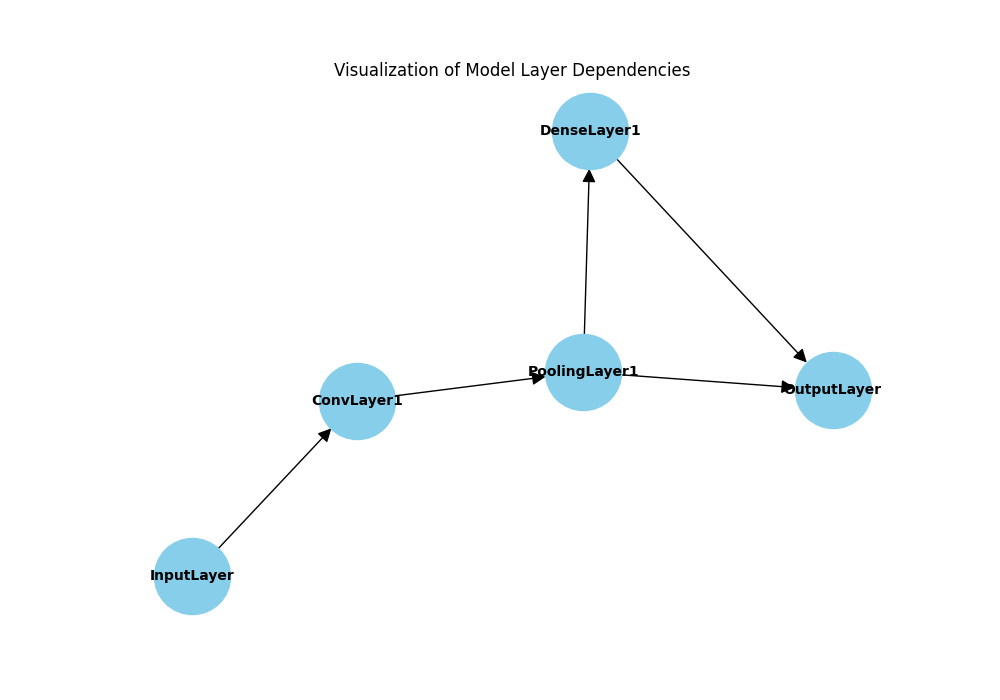
Abstract data structures and algorithms become much easier to understand when they can be visualized. Using libraries like matplotlib and networkx, we can create visual representations of graphs, helping to clarify their structure and the behavior of traversal algorithms.
The following example visualizes the model_graph we created earlier, showing the layers and their connections. This kind of visualization is invaluable for debugging complex model architectures.
        graph TD
            A[Start BFS with a given root node] --> B{Is root node valid?};
            B -- Yes --> C[1- Create a queue];
            B -- No --> End_Error[End: Invalid Node];
            C --> D[2- Create a 'visited' set];
            D --> E[3- Add root node to queue and 'visited' set];
            E --> F{Is the queue empty?};
            F -- No --> G["4- Dequeue a node (call it 'current')"];
            G --> H["5- Process 'current' node<br> (e.g., add to result list)"];
            H --> I[6- For each neighbor of 'current'];
            I --> J{Is neighbor in 'visited' set?};
            J -- No --> K[7- Add neighbor to 'visited' set];
            K --> L[8- Enqueue the neighbor];
            L --> F;
            J -- Yes --> I;
            I -- All neighbors checked --> F;
            F -- Yes --> End_Success[End: Traversal Complete];

            %% Styling
            style A fill:#283044,stroke:#283044,stroke-width:2px,color:#ebf5ee
            style B fill:#f39c12,stroke:#f39c12,stroke-width:1px,color:#283044
            style F fill:#f39c12,stroke:#f39c12,stroke-width:1px,color:#283044
            style J fill:#f39c12,stroke:#f39c12,stroke-width:1px,color:#283044
            style C fill:#78a1bb,stroke:#78a1bb,stroke-width:1px,color:#283044
            style D fill:#78a1bb,stroke:#78a1bb,stroke-width:1px,color:#283044
            style E fill:#78a1bb,stroke:#78a1bb,stroke-width:1px,color:#283044
            style G fill:#78a1bb,stroke:#78a1bb,stroke-width:1px,color:#283044
            style H fill:#78a1bb,stroke:#78a1bb,stroke-width:1px,color:#283044
            style I fill:#78a1bb,stroke:#78a1bb,stroke-width:1px,color:#283044
            style K fill:#78a1bb,stroke:#78a1bb,stroke-width:1px,color:#283044
            style L fill:#78a1bb,stroke:#78a1bb,stroke-width:1px,color:#283044
            style End_Success fill:#2d7a3d,stroke:#2d7a3d,stroke-width:2px,color:#ebf5ee
style End_Error fill:#d63031,stroke:#d63031,stroke-width:2px,color:#ebf5ee# A complete, working example of visualizing a graph with networkx and matplotlib
import networkx as nx
import matplotlib.pyplot as plt
# Using the model_graph from the first example
# model_graph = Graph() ... (assume it's defined as before)
# Create a NetworkX DiGraph object from our custom graph's adjacency list
G = nx.DiGraph(model_graph.adj_list)
plt.figure(figsize=(10, 7))
plt.title("Visualization of Model Layer Dependencies")
# Use a layout algorithm to position the nodes
pos = nx.spring_layout(G, seed=42)
# Draw the graph
nx.draw(G, pos, with_labels=True, node_size=3000, node_color='skyblue',
font_size=10, font_weight='bold', arrowsize=20)
plt.show()
Computational Exercises
To solidify understanding, hands-on implementation is key. These exercises bridge theory and practice.
Exercise 1: Performance Comparison
Manually calculate the number of operations required to find an element in a list of 16 items using linear search versus binary search in the worst-case scenario. Then, write a Python script using the time module to measure the actual execution time difference on a large sorted list (e.g., 10 million elements).
Manual Calculation:
- Linear Search (worst case): Checks every element, so 16 operations.
- Binary Search (worst case): \(\log_2(16) = 4\) operations.
Library-based Implementation:
import time
import random

# Prepare a large, sorted list
n = 10_000_000
large_sorted_list = list(range(n))
# The element to search for (worst case for linear search)
target = n - 1

# --- Linear Search ---
start_time = time.perf_counter()
try:
    large_sorted_list.index(target)
    end_time = time.perf_counter()
    print(f"Linear search time: {end_time - start_time:.6f} seconds")
except ValueError:
    print("Target not found.")


# --- Binary Search (using the 'bisect' module) ---
import bisect

start_time = time.perf_counter()
# bisect_left finds the insertion point, which is equivalent to a search
index = bisect.bisect_left(large_sorted_list, target)
end_time = time.perf_counter()
# Verify if the element is actually at that index
if index < n and large_sorted_list[index] == target:
    print(f"Binary search time: {end_time - start_time:.6f} seconds")
else:
    print("Target not found.")
Outputs:
Linear search time: 0.059601 seconds
Binary search time: 0.000005 seconds
Real-World Problem Applications
Let’s apply these concepts to a common problem in recommendation systems: finding “similar” users. We can use a defaultdict to create an inverted index mapping items to the users who have liked them. Then, we can use collections.Counter to find users who have liked the same items as a target user.
from collections import defaultdict, Counter

# Sample data: user -> set of liked movie IDs
user_likes = {
    'Alice': {'m1', 'm2', 'm4'},
    'Bob': {'m2', 'm3', 'm5'},
    'Charlie': {'m1', 'm4', 'm6'},
    'Diana': {'m2', 'm3', 'm7'},
    'Eve': {'m1', 'm4'},
}

# --- Build an inverted index: movie -> list of users who liked it ---
movie_fans = defaultdict(list)
for user, movies in user_likes.items():
    for movie in movies:
        movie_fans[movie].append(user)

print("--- Inverted Index (Movie -> Fans) ---")
print(dict(movie_fans))

# --- Find users with similar tastes to 'Alice' ---
target_user = 'Alice'
similar_users = Counter()

# For each movie Alice likes...
for movie in user_likes[target_user]:
    # ...find other users who also liked that movie.
    for user in movie_fans[movie]:
        if user != target_user:
            similar_users[user] += 1

print(f"\n--- Users similar to {target_user} (by shared movie likes) ---")
# The most_common() method returns a list of (user, count) tuples
print(similar_users.most_common())
Outputs:
--- Inverted Index (Movie -> Fans) ---
{'m2': ['Alice', 'Bob', 'Diana'], 'm1': ['Alice', 'Charlie', 'Eve'], 'm4': ['Alice', 'Charlie', 'Eve'], 'm3': ['Bob', 'Diana'], 'm5': ['Bob'], 'm6': ['Charlie'], 'm7': ['Diana']}

--- Users similar to Alice (by shared movie likes) ---
[('Charlie', 2), ('Eve', 2), ('Bob', 1), ('Diana', 1)]
This example demonstrates how choosing the right data structures (defaultdict, Counter) leads to clean, efficient, and readable code that solves a real-world AI problem.
Industry Applications and Case Studies
The advanced Python concepts covered in this chapter are not merely academic; they are the bedrock of production AI systems at leading technology companies. At Netflix, recommendation algorithms rely heavily on graph-based data structures to model the complex relationships between users, content, and viewing history. Efficiently traversing these massive graphs to generate personalized recommendations in real-time requires optimized algorithms and data structures far beyond simple lists and dictionaries. The engineering challenge involves not just the algorithm’s theoretical complexity but also its implementation in a distributed environment, where data is sharded across many machines. The choice of data representation and traversal strategy directly impacts latency and computational cost, which in turn affects user experience and operational expenses.
Google’s search engine is another prime example. The web is modeled as a colossal directed graph where web pages are nodes and hyperlinks are edges. Algorithms like PageRank, which determines the importance of a page, are fundamentally graph algorithms. To support features like instant search and autocomplete, Google employs highly specialized tree-like data structures, such as Tries (or more advanced variants like Radix Tries), to search through trillions of potential queries in milliseconds. The implementation must be incredibly memory-efficient and computationally optimized to handle the immense scale and speed requirements.
In the financial sector, high-frequency trading (HFT) firms use priority queues, implemented with heaps, to manage the order book of a stock exchange. Incoming buy and sell orders must be processed based on price and time priority. The ability to add new orders and retrieve the highest-priority order in \(O(\log n)\) time is critical for executing trades faster than the competition, where microseconds can translate into millions of dollars. These firms invest heavily in optimizing these fundamental data structures and algorithms, often going beyond standard library implementations to shave off every possible nanosecond of latency. These cases illustrate that a deep understanding of data structures and algorithms is a key differentiator in building competitive, high-performance AI and data-driven systems.
Best Practices and Common Pitfalls
Mastering advanced Python for AI involves not only knowing what tools to use but also how and when to use them effectively. A primary best practice is to always choose the right data structure for the job. Before defaulting to a list, analyze the access patterns of your problem. If you need frequent additions or removals from the beginning of a sequence, a deque is the superior choice. If you need fast lookups by a key, a dict or set is appropriate. This conscious choice can prevent significant performance bottlenecks down the line. Another key practice is to leverage the standard library. The collections, itertools, and heapq modules are written in C, highly optimized, and thoroughly tested. Re-implementing their functionality is often a source of bugs and performance issues.
A common pitfall is premature optimization. While understanding Big O is crucial, spending hours optimizing a non-critical part of a data pipeline that only runs once a day is an inefficient use of development time. Use profiling tools like cProfile to identify the actual bottlenecks in your code before you start optimizing. Another mistake is creating monolithic, inflexible classes in object-oriented design. AI models and systems evolve rapidly. Design your classes to be modular and adhere to the Single Responsibility Principle. A class should do one thing and do it well. This makes the system easier to test, debug, and extend.
In functional data pipelines, a common error is to introduce subtle side effects into functions that are assumed to be pure. A function that modifies a global variable or an input list in-place can lead to unpredictable behavior that is incredibly difficult to debug. Strive to make your data transformation functions pure and operate on immutable data where possible. Finally, neglecting to write tests for your custom data structures and algorithms is a recipe for disaster. The logic can be complex, and edge cases are numerous. A robust test suite is essential for ensuring the correctness and reliability of the foundational code upon which your AI models are built.
Tip: Profile your code before you optimize. The
cProfilemodule can show you exactly where your program is spending its time, ensuring you focus your efforts where they will have the most impact.
Hands-on Exercises
These exercises are designed to reinforce the concepts from this chapter, progressing from fundamental application to more complex design.
- Deque for Log Processing (Basic): You are processing a stream of application logs and need to keep track of the last 100 log entries to detect recent error patterns. Write a Python function that takes a new log entry and a
dequeof existing entries. The function should add the new entry and ensure thedequenever holds more than 100 entries. Compare the clarity and theoretical performance of this approach to using a standardlistand slicing. - Building a Weighted Graph for Pathfinding (Intermediate): Extend the
Graphclass from the practical examples section to support weighted edges. Modify theadd_edgemethod to accept a third argument,weight. Then, implement Dijkstra’s algorithm to find the shortest path between two nodes in the weighted graph. Use a min-heap (heapq) as the priority queue for efficiency. Create a sample graph representing cities and distances to test your implementation. - OOP Design for a Simple ML Model (Advanced/Team): Design a set of Python classes to represent a K-Nearest Neighbors (KNN) classifier. Your design should include:
- A
KNNClassifierclass with methods likefit(X, y)andpredict(X_test). - The
fitmethod should store the training data. - The
predictmethod should, for each test point, calculate the distance to all training points, find theknearest neighbors, and predict the majority class among them. - Encapsulate the distance metric (e.g., Euclidean distance) in its own helper function or method.
- Discuss as a team how you could use inheritance to allow the classifier to easily switch between different distance metrics (e.g., Euclidean, Manhattan).
- A
Tools and Technologies
To effectively apply the concepts in this chapter, proficiency with several tools and libraries is essential. The cornerstone is, of course, a modern version of Python (3.11+), which includes numerous performance improvements and syntax enhancements. The Python standard library is your first and most important tool; modules like collections, itertools, functools, and heapq provide the high-performance building blocks for many algorithms. For performance analysis, Python’s built-in cProfile and timeit modules are indispensable for identifying bottlenecks and comparing the speed of different implementations.
For numerical and data-heavy tasks, the core scientific computing libraries are non-negotiable. NumPy provides the ndarray object, a highly efficient multi-dimensional array, and a vast collection of mathematical functions. Pandas builds on NumPy to offer data structures like the DataFrame, which is essential for data manipulation and analysis. When working with graphs, NetworkX is the standard library for the creation, manipulation, and study of the structure, dynamics, and functions of complex networks. For visualization, Matplotlib and Seaborn are the go-to libraries for creating static, animated, and interactive visualizations, which are crucial for understanding data and algorithm behavior. A modern IDE like VS Code or PyCharm with integrated debugging, linting, and testing capabilities will dramatically improve your productivity and code quality.
Summary
This chapter provided a deep dive into the advanced Python programming skills that are foundational to modern AI engineering. We moved beyond basic syntax to explore how data structures, algorithms, and programming paradigms are applied to build efficient, scalable, and maintainable AI systems.
- Key Concepts Recap: We established the importance of the Pythonic mindset for writing readable code, analyzed algorithmic efficiency using Big O notation, and explored advanced data structures like deques, heaps, graphs, and trees. We also contrasted the Object-Oriented and Functional programming paradigms and their respective roles in AI application design.
- Practical Skills Gained: You have learned to implement these data structures and algorithms from scratch, apply them to solve real-world AI problems like autocomplete and recommendation systems, and visualize their behavior.
- Connection to Future Topics: The principles of OOP are the basis for understanding deep learning frameworks like PyTorch and TensorFlow. The functional programming concepts for data pipelines are directly applicable to big data processing with tools like Apache Spark.
- Real-World Applicability: The skills learned here are directly transferable to a professional AI engineering role, where performance, scalability, and code quality are paramount. Mastering these fundamentals is a prerequisite for tackling complex challenges in any AI domain.
Further Reading and Resources
- “Fluent Python, 2nd Edition” by Luciano Ramalho: An essential, comprehensive guide to writing effective, idiomatic Python code. It covers many of the data structures and concepts discussed in this chapter in great detail.
- Python Official Documentation – Data Structures: The official documentation is the ultimate source of truth for the standard library, including the
collectionsmodule. (https://docs.python.org/3/tutorial/datastructures.html) - “Problem Solving with Algorithms and Data Structures using Python” by Miller and Ranum: An interactive online textbook that provides a great introduction to the topic with runnable code examples.
- GeeksforGeeks – Algorithms: A vast and popular resource with clear explanations and implementations of countless algorithms and data structures in multiple languages, including Python.
- NetworkX Official Documentation: For anyone working with graph data, the official documentation and tutorial for the NetworkX library is the best place to start. (https://networkx.org/documentation/stable/)
- Real Python (realpython.com): A fantastic resource with high-quality tutorials on a wide range of Python topics, from beginner to advanced, including performance optimization and data structures.
- “Introduction to Algorithms, 3rd Edition” by Cormen, Leiserson, Rivest, and Stein (CLRS): The definitive academic textbook on algorithms. While language-agnostic, it provides the rigorous theoretical foundation for all the concepts discussed.
Glossary of Terms
- Algorithm: A finite sequence of well-defined, computer-implementable instructions, typically to solve a class of problems or to perform a computation.
- Big O Notation: A mathematical notation that describes the limiting behavior of a function when the argument tends towards a particular value or infinity. In computer science, it is used to classify algorithms according to how their run time or space requirements grow as the input size grows.
- Data Structure: A particular way of organizing and storing data in a computer so that it can be accessed and modified efficiently. Examples include lists, graphs, and trees.
- Deque (Double-Ended Queue): A queue-like data structure that supports adding and removing elements from both ends with \(O(1)\) time complexity.
- Functional Programming (FP): A programming paradigm where programs are constructed by applying and composing functions. It treats computation as the evaluation of mathematical functions and avoids changing-state and mutable data.
- Graph: A data structure consisting of a set of vertices (or nodes) and a set of edges that connect pairs of vertices.
- Heap: A specialized tree-based data structure that satisfies the heap property: in a min-heap, for any given node C, if P is a parent node of C, then the key of P is less than or equal to the key of C. It is commonly used to implement priority queues.
- Object-Oriented Programming (OOP): A programming paradigm based on the concept of “objects”, which can contain data in the form of fields (often known as attributes or properties), and code, in the form of procedures (often known as methods).
- Trie: A tree-like data structure, also known as a prefix tree, that is used to store a dynamic set of strings.
