
Chapter 35: Data Transformation: Scaling, Normalization, and Encoding
Chapter Objectives
Upon completing this chapter, students will be able to:
- Understand the theoretical foundations and mathematical principles behind common data transformation techniques, including scaling, normalization, and encoding.
- Analyze datasets to identify the appropriate transformation strategies based on data characteristics and the requirements of specific machine learning algorithms.
- Implement various scaling methods (Standardization, Min-Max, Robust Scaling) and encoding techniques (One-Hot, Ordinal) using modern Python libraries like scikit-learn and NumPy.
- Design and build robust data preprocessing pipelines that correctly apply transformations to training and testing data to prevent data leakage.
- Evaluate the impact of different data transformations on the performance, convergence, and stability of machine learning models.
- Optimize data preprocessing workflows for large-scale datasets, considering computational efficiency and the trade-offs between different techniques.
Introduction
In the intricate process of developing high-performance AI systems, raw data is rarely, if ever, suitable for direct consumption by machine learning algorithms. The journey from raw, unstructured information to actionable insight is paved with a series of critical preparatory steps, collectively known as data preprocessing. Within this domain, data transformation stands as a cornerstone practice, fundamentally reshaping the data’s structure and values to meet the mathematical assumptions and operational requirements of learning algorithms. This chapter delves into the essential techniques of data transformation—scaling, normalization, and encoding—that are indispensable in the toolkit of any modern AI engineer.
The importance of these transformations cannot be overstated. Many powerful algorithms, from the classic Support Vector Machines (SVMs) to the deep neural networks that power today’s most advanced AI, are sensitive to the scale and distribution of their input features. An unscaled feature with a large range can disproportionately influence a model’s learning process, leading to slower convergence and suboptimal performance. Similarly, categorical data, such as product categories or user locations, must be converted into a numerical format before it can be processed. This chapter will equip you with the knowledge to navigate these challenges, providing a deep dive into not just the “how” but, more critically, the “why” and “when” of applying these techniques. We will explore the mathematical underpinnings of each method, implement them in practical Python examples, and situate their use within the broader context of building production-ready MLOps pipelines. By the end of this chapter, you will have moved beyond treating preprocessing as a mechanical checklist and will instead approach it as a strategic component of model design and optimization.
graph TB
    subgraph "Data Transformation Pipeline"
    direction TB
        A[Start: Raw Data] --> B{Identify Feature Types};
        B --> C[Numerical Features];
        B --> D[Categorical Features];

        C --> E{Assess Distribution & Outliers};
        E -->|Normal Distribution| F[StandardScaler];
        E -->|Contains Outliers| G[RobustScaler];
        E -->|Bounded Range Needed| H[MinMaxScaler];

        D --> I{Assess Data Type};
        I -->|Nominal Data| J[OneHotEncoder];
        I -->|Ordinal Data| K[OrdinalEncoder];

        F --> L[Scaled Numerical Data];
        G --> L;
        H --> L;
        J --> M[Encoded Categorical Data];
        K --> M;

        L --> N[Combine Features];
        M --> N;

        N --> O[End: Model-Ready Data];
    end

    %% Styling
    style A fill:#283044,stroke:#283044,stroke-width:2px,color:#ebf5ee
    style O fill:#2d7a3d,stroke:#2d7a3d,stroke-width:2px,color:#ebf5ee
    style B fill:#f39c12,stroke:#f39c12,stroke-width:1px,color:#283044
    style E fill:#f39c12,stroke:#f39c12,stroke-width:1px,color:#283044
    style I fill:#f39c12,stroke:#f39c12,stroke-width:1px,color:#283044
    style C fill:#9b59b6,stroke:#9b59b6,stroke-width:1px,color:#ebf5ee
    style D fill:#9b59b6,stroke:#9b59b6,stroke-width:1px,color:#ebf5ee
    style L fill:#9b59b6,stroke:#9b59b6,stroke-width:1px,color:#ebf5ee
    style M fill:#9b59b6,stroke:#9b59b6,stroke-width:1px,color:#ebf5ee
    style F fill:#e74c3c,stroke:#e74c3c,stroke-width:1px,color:#ebf5ee
    style G fill:#e74c3c,stroke:#e74c3c,stroke-width:1px,color:#ebf5ee
    style H fill:#e74c3c,stroke:#e74c3c,stroke-width:1px,color:#ebf5ee
    style J fill:#e74c3c,stroke:#e74c3c,stroke-width:1px,color:#ebf5ee
    style K fill:#e74c3c,stroke:#e74c3c,stroke-width:1px,color:#ebf5ee
    style N fill:#78a1bb,stroke:#78a1bb,stroke-width:1px,color:#283044
Technical Background
The Rationale for Data Transformation
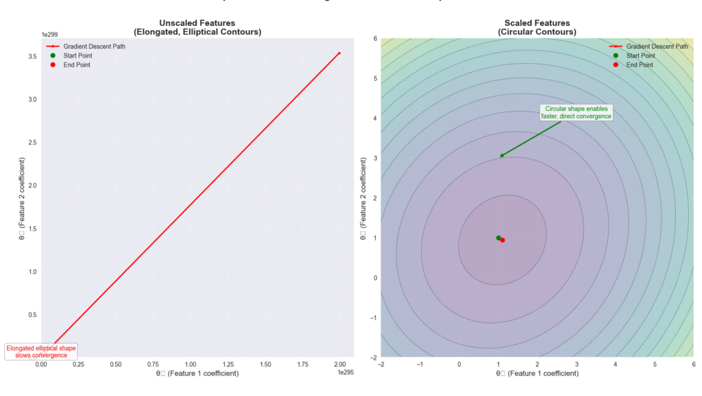
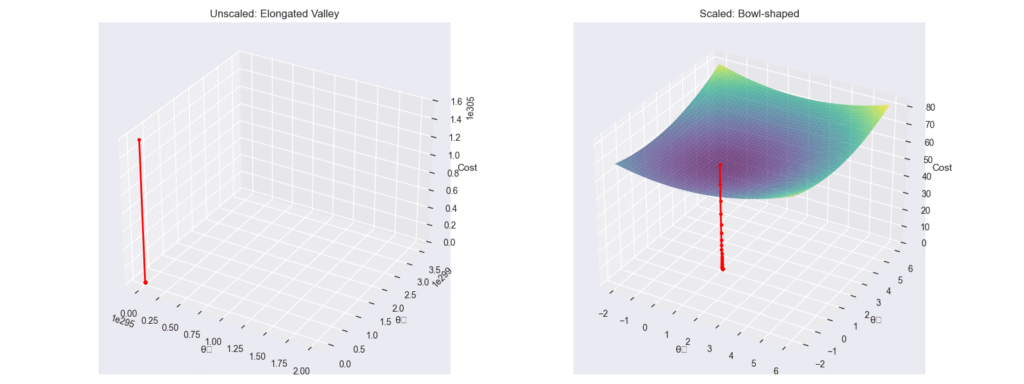
The core objective of a machine learning model is to learn a mapping function from input features to output targets. The effectiveness of this learning process is profoundly influenced by the landscape of the input data. Imagine trying to train a model to predict housing prices using two features: the number of rooms (ranging from 1 to 10) and the square footage of the property (ranging from 500 to 10,000). During the optimization process, algorithms that use gradient descent will find that the gradients associated with square footage are orders of magnitude larger than those for the number of rooms. This disparity can cause the optimization process to oscillate inefficiently or converge very slowly, as the model struggles to balance the contributions of these differently scaled features. Data transformation addresses this by bringing all features onto a common scale, ensuring that no single feature dominates the learning process simply due to its magnitude.
Beyond scale, many algorithms operate on assumptions about the data’s distribution. Linear models, for instance, often perform better when the input features are normally distributed. While transformation cannot magically change the underlying nature of the data, techniques like logarithmic or Box-Cox transformations can help mitigate severe skewness, making the data more amenable to these models. Furthermore, the world is not purely numerical. Categorical information is ubiquitous, and transforming it into a meaningful numerical representation is a non-trivial task that directly impacts a model’s ability to learn from this data. Choosing the wrong encoding scheme can introduce artificial ordinal relationships where none exist, misleading the model and degrading its performance. Therefore, data transformation is not merely a janitorial task; it is a fundamental aspect of feature engineering that directly shapes a model’s ability to perceive and learn from the data provided.
Feature Scaling and Standardization
Feature scaling is the process of adjusting the range of numerical features. It is a critical step for algorithms that compute distances between data points or use gradient-based optimization. The two most prominent methods for scaling are Standardization and Min-Max Scaling, often referred to as Normalization, though the term can be ambiguous.
Standardization (Z-score Scaling)
Standardization, also known as Z-score scaling, is a technique that transforms features to have a mean of 0 and a standard deviation of 1. This is achieved by subtracting the feature’s mean (\(\mu\)) from each data point (\(x\)) and then dividing by the feature’s standard deviation (\(\sigma\)). The formula for a single data point is:\[z = \frac{x – \mu}{\sigma}\]
The resulting value, \(z\), represents the number of standard deviations a data point is from the mean. This transformation centers the data around the origin and scales it based on its own variance. A key advantage of standardization is that it does not bind the data to a specific range, which makes it less sensitive to outliers compared to other scaling methods. If a dataset contains significant outliers, standardization will scale them down, but they will remain as distinct values far from the mean. This property makes it a robust choice for a wide variety of algorithms, including Support Vector Machines (SVMs) with Radial Basis Function (RBF) kernels, Principal Component Analysis (PCA), and linear models like Logistic Regression and Linear Regression, as it helps the gradient descent optimizer converge more quickly and reliably.
Min-Max Scaling
Min-Max scaling is a transformation that rescales a feature to a fixed range, typically between 0 and 1. It achieves this by subtracting the minimum value (\(x_{min}\)) in the feature from each data point and then dividing by the range of the feature (the difference between the maximum and minimum values, \(x_{max} – x_{min}\)). The formula is:\[x_{scaled} = \frac{x – x_{min}}{x_{max} – x_{min}}\]
The primary benefit of Min-Max scaling is that it guarantees all features will have the exact same scale, which can be beneficial for algorithms that are not based on distributions, such as k-Nearest Neighbors (k-NN), and for certain types of neural networks where activation functions like Sigmoid or Tanh expect inputs within a bounded range. However, its major drawback is its sensitivity to outliers. A single extreme value in the dataset will define the new maximum or minimum, which can compress the rest of the data into a very small sub-range, potentially hindering the model’s ability to learn from the variance in the “inlier” data. Therefore, it is typically recommended when the data is known to be bounded within a certain range or when outliers have already been handled.
Robust Scaling
When a dataset contains a significant number of outliers, both Standardization and Min-Max scaling can be compromised. Robust Scaling offers a powerful alternative by using statistics that are less sensitive to extreme values. Instead of the mean and standard deviation, it uses the median and the interquartile range (IQR). The IQR is the range between the first quartile (25th percentile, \(Q_1\)) and the third quartile (75th percentile, \(Q_3\)). The transformation is performed by subtracting the median from each data point and dividing by the IQR:\[x_{scaled} = \frac{x – \text{median}(x)}{Q_3(x) – Q_1(x)}\]
By using the median and IQR, this method effectively ignores the influence of outliers when scaling the data. The bulk of the data, centered around the median, is scaled into a compact range, while the outliers remain as extreme values but do not dictate the scaling parameters for the rest of the data. This makes Robust Scaling an excellent choice for datasets with measurement errors or anomalies that should not unduly influence the feature scaling process. It provides a reliable way to prepare data for a wide range of algorithms in scenarios where data cleanliness cannot be fully guaranteed.
Comparison of Feature Scaling Techniques
| Technique | Formula | Key Characteristics | Best For | Sensitivity to Outliers |
|---|---|---|---|---|
| Standardization (Z-score Scaling) |
z = (x - μ) / σ |
Transforms data to have a mean of 0 and a standard deviation of 1. Does not bind data to a specific range. | Algorithms that assume a Gaussian distribution (e.g., Linear Regression, Logistic Regression, SVMs). General-purpose default. | Low. Outliers are scaled down but remain in the tails of the distribution. |
| Min-Max Scaling (Normalization) |
x_scaled = (x - x_min) / (x_max - x_min) |
Scales data to a fixed range, typically [0, 1]. All features will have the exact same scale. | Algorithms that do not assume a specific distribution (e.g., k-NN). Neural networks with activation functions sensitive to input range (e.g., Sigmoid). | High. A single outlier can squash the majority of the inlier data into a very small range. |
| Robust Scaling | x_scaled = (x - median) / IQR |
Uses the median and Interquartile Range (IQR), making it robust to outliers. Centers data around the median. | Datasets containing significant outliers or measurement errors. When data cleanliness cannot be guaranteed. | Very Low. The scaling parameters (median, IQR) are not influenced by extreme values. |
Encoding Categorical Variables
Machine learning algorithms are fundamentally mathematical, operating on numbers and vectors. They cannot directly interpret categorical data, such as ‘Red’, ‘Green’, ‘Blue’ or ‘USA’, ‘Canada’, ‘Mexico’. Therefore, a crucial step in data transformation is encoding these non-numeric variables into a numerical format. The choice of encoding strategy depends heavily on the nature of the categorical data itself.
Nominal vs. Ordinal Data
The first step in choosing an encoding method is to distinguish between nominal and ordinal data. Ordinal data has an inherent, meaningful order or ranking among its categories. For example, clothing sizes (‘Small’, ‘Medium’, ‘Large’) or customer satisfaction ratings (‘Poor’, ‘Average’, ‘Good’, ‘Excellent’) have a clear hierarchy. ‘Large’ is greater than ‘Medium’, and ‘Excellent’ is better than ‘Good’. Nominal data, on the other hand, consists of categories with no intrinsic order or ranking. Examples include colors (‘Red’, ‘Green’, ‘Blue’), countries (‘USA’, ‘Canada’, ‘Mexico’), or types of pets (‘Dog’, ‘Cat’, ‘Fish’). There is no inherent sense in which ‘Blue’ is greater than ‘Red’ or ‘Canada’ is greater than ‘USA’. This distinction is critical because applying an encoding method that implies an order to nominal data can mislead the learning algorithm into finding non-existent relationships, thereby degrading its performance.
One-Hot Encoding for Nominal Data
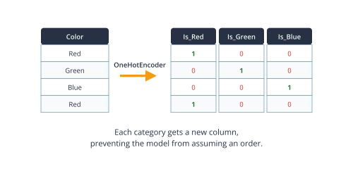
For nominal data, the most common and effective encoding technique is One-Hot Encoding. This method transforms each category into a new binary feature, or “dummy variable.” For a feature with \(k\) distinct categories, One-Hot Encoding creates \(k\) new columns. For each data point, the column corresponding to its category is set to 1, and all other \(k-1\) columns are set to 0. For example, a ‘Color’ feature with categories ‘Red’, ‘Green’, and ‘Blue’ would be transformed into three new features: is_Red, is_Green, and is_Blue. A data point with the value ‘Red’ would be represented as [1, 0, 0].
This approach ensures that no ordinal relationship is implied between the categories. The model sees each category as an independent entity. However, a potential issue arises known as the “dummy variable trap,” where the new features are perfectly multicollinear (e.g., if we know is_Red is 0 and is_Green is 0, we know is_Blue must be 1). To avoid this, it is standard practice to drop one of the new columns, representing its information implicitly. The main drawback of One-Hot Encoding is that it can lead to a significant increase in the number of features (the “curse of dimensionality”) if the original categorical variable has high cardinality (many unique categories), which can increase computational cost and sometimes lead to overfitting.
Ordinal Encoding for Ordinal Data
When dealing with ordinal data, a simpler and more appropriate method is Ordinal Encoding (often referred to as Label Encoding in some contexts, though the terms can have slightly different implementations). This technique maps each category to a unique integer based on its rank. For example, with the sizes ‘Small’, ‘Medium’, and ‘Large’, we could map them to 0, 1, and 2, respectively. This preserves the ordinal relationship in the data: \(2 > 1 > 0\).
This method is computationally efficient and avoids adding new dimensions to the data. However, it should be used with extreme caution and only on genuinely ordinal features. Applying it to nominal data would be a critical mistake. For instance, if we encoded ‘USA’ as 0, ‘Canada’ as 1, and ‘Mexico’ as 2, the model would incorrectly assume that ‘Canada’ is somehow halfway between ‘USA’ and ‘Mexico’, and that ‘Mexico’ is twice the value of ‘Canada’. Such arbitrary numerical assignments can introduce noise and bias, leading the model to learn spurious patterns and ultimately fail to generalize well to new data.
Comparison of Categorical Encoding Techniques
| Technique | Data Type | How It Works | Pros | Cons |
|---|---|---|---|---|
| One-Hot Encoding | Nominal (No inherent order, e.g., Colors, Countries) |
Creates a new binary (0/1) column for each unique category. | Avoids creating false ordinal relationships. Model can learn the independent effect of each category. | Can significantly increase dimensionality (curse of dimensionality) if cardinality is high. |
| Ordinal Encoding | Ordinal (Inherent order, e.g., Sizes: S, M, L) |
Maps each category to a unique integer based on its rank (e.g., S=0, M=1, L=2). | Preserves the ordinal nature of the data. Computationally efficient; does not add dimensions. | Critical: Should never be used on nominal data as it will introduce a false and misleading order. |
Warning: Always fit scalers and encoders on the training data only. Then, use the same fitted object to transform both the training data and the test/validation data. Fitting on the entire dataset before splitting would cause data leakage, where information from the test set bleeds into the training process, leading to an overly optimistic evaluation of model performance.
sequenceDiagram
    actor User as AI Engineer
    participant Data as Raw Data
    participant Scaler as StandardScaler
    participant TrainSet as Training Data
    participant TestSet as Testing Data
    participant Model as ML Model

    rect rgb(235, 245, 238)
        Note over User, Model: Correct Workflow (No Data Leakage)
        User->>Data: 1. Split Data First
        Data->>TrainSet: Training Set (80%)
        Data->>TestSet: Testing Set (20%)
        User->>Scaler: 2. Create Scaler Instance
        User->>Scaler: 3. Fit Scaler on Training Data ONLY
        TrainSet->>Scaler: Learn scaling parameters (mean, std)
        Scaler->>TrainSet: 4. Transform Training Data
        TrainSet->>TrainSet: Scaled Training Data
        Scaler->>TestSet: 5. Transform Testing Data (same params)
        TestSet->>TestSet: Scaled Testing Data
        User->>Model: 6. Train Model on Scaled Train Data
        User->>Model: 7. Evaluate on Scaled Test Data
        Note right of Model: Valid performance estimate
    end

    rect rgb(255, 221, 221)
        Note over User, Model: Incorrect Workflow (Data Leakage!)
        User->>Scaler: 1. Fit Scaler on ALL Data
        Data->>Scaler: Learn params from entire dataset
        User->>Data: 2. Split Data After Scaling
        Data->>TrainSet: Training Set
        Data->>TestSet: Testing Set
        Scaler->>TrainSet: 3. Transform Training Data
        Scaler->>TestSet: 4. Transform Testing Data
        User->>Model: 5. Train Model
        User->>Model: 6. Evaluate Model
        Note right of Model: Unrealistically optimistic<br/>performance estimate!
    end
Practical Examples and Implementation
This section translates the theoretical concepts of data transformation into practical, executable Python code. We will leverage the power of scikit-learn, NumPy, and pandas to perform scaling and encoding, and use matplotlib and seaborn to visualize the results, reinforcing the intuition behind each technique.
Implementing Scaling Techniques
Let’s start with a synthetic dataset to demonstrate the effects of different scaling methods. We’ll create a dataset with two features that have different scales and distributions.
import numpy as np
import pandas as pd
from sklearn.preprocessing import StandardScaler, MinMaxScaler, RobustScaler
import matplotlib.pyplot as plt
import seaborn as sns

# Generate synthetic data
np.random.seed(42)
data = pd.DataFrame({
    'Feature1': np.random.normal(loc=50, scale=10, size=1000),
    'Feature2': np.random.exponential(scale=100, size=1000) + 200,
})

# Add some outliers to Feature2
data.loc[990:] = data.loc[990:] * 5

print("Original Data Description:")
print(data.describe())

# --- Visualization of Original Data ---
plt.figure(figsize=(15, 5))

plt.subplot(1, 2, 1)
sns.histplot(data['Feature1'], kde=True, bins=30)
plt.title('Original Distribution of Feature 1')

plt.subplot(1, 2, 2)
sns.histplot(data['Feature2'], kde=True, bins=30)
plt.title('Original Distribution of Feature 2 (with outliers)')

plt.tight_layout()
plt.show()
Outputs:
Original Data Description:
          Feature1     Feature2
count  1000.000000  1000.000000
mean     52.129109   311.631666
std      21.998944   153.008795
min      17.587327   200.322345
25%      43.625247   229.024888
50%      50.404177   273.309444
75%      56.760141   342.554036
max     339.884326  2779.499450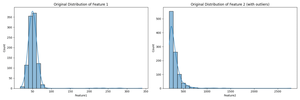
The output shows that Feature1 is normally distributed around 50, while Feature2 is exponentially distributed with a much larger scale and significant outliers.
Applying Scalers
Now, let’s apply our three main scalers and observe their effects.
# Initialize scalers
std_scaler = StandardScaler()
minmax_scaler = MinMaxScaler()
robust_scaler = RobustScaler()

# Fit and transform the data
data_std = std_scaler.fit_transform(data)
data_minmax = minmax_scaler.fit_transform(data)
data_robust = robust_scaler.fit_transform(data)

# Convert back to DataFrame for easier plotting
df_std = pd.DataFrame(data_std, columns=['Feature1', 'Feature2'])
df_minmax = pd.DataFrame(data_minmax, columns=['Feature1', 'Feature2'])
df_robust = pd.DataFrame(data_robust, columns=['Feature1', 'Feature2'])

# --- Visualization of Scaled Data ---
fig, axes = plt.subplots(3, 2, figsize=(15, 15))
fig.suptitle('Comparison of Scaling Techniques', fontsize=16)

# Standard Scaler
sns.histplot(df_std['Feature1'], kde=True, ax=axes[0, 0]).set_title('Standard Scaler - Feature 1')
sns.histplot(df_std['Feature2'], kde=True, ax=axes[0, 1]).set_title('Standard Scaler - Feature 2')

# Min-Max Scaler
sns.histplot(df_minmax['Feature1'], kde=True, ax=axes[1, 0]).set_title('Min-Max Scaler - Feature 1')
sns.histplot(df_minmax['Feature2'], kde=True, ax=axes[1, 1]).set_title('Min-Max Scaler - Feature 2')

# Robust Scaler
sns.histplot(df_robust['Feature1'], kde=True, ax=axes[2, 0]).set_title('Robust Scaler - Feature 1')
sns.histplot(df_robust['Feature2'], kde=True, ax=axes[2, 1]).set_title('Robust Scaler - Feature 2')

plt.tight_layout(rect=[0, 0.03, 1, 0.95])
plt.show()
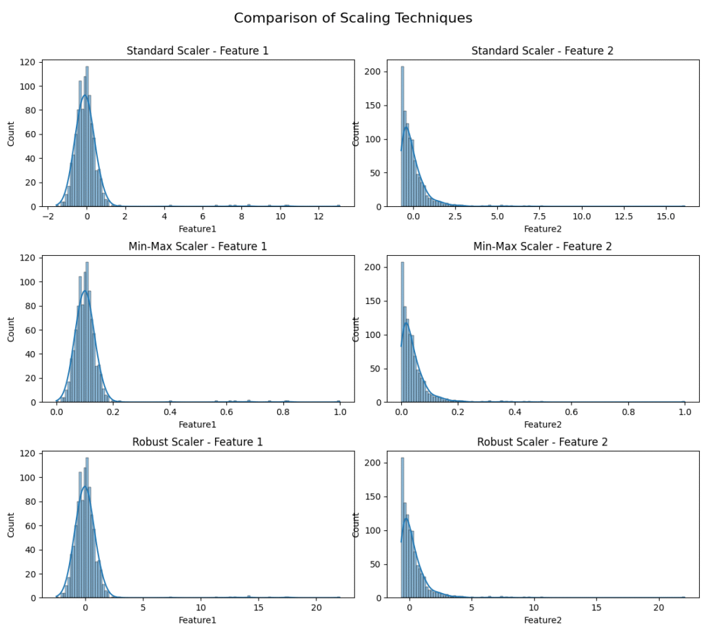
From the visualizations, we can draw clear conclusions. StandardScaler centers the data around 0. MinMaxScaler scales the data to the [0, 1] range, but for Feature2, the outliers cause the vast majority of the data to be squashed into a tiny portion of that range. RobustScaler handles the outliers in Feature2 much more effectively, scaling the bulk of the data to a reasonable range while the outliers remain far from the center. This practical example vividly illustrates the importance of choosing a scaler appropriate for the data’s characteristics.
Implementing Encoding Techniques
Next, let’s work with a dataset containing categorical features to demonstrate encoding.
from sklearn.preprocessing import OneHotEncoder, OrdinalEncoder

# Create a sample dataset
df_categorical = pd.DataFrame({
    'Color': ['Red', 'Blue', 'Green', 'Blue', 'Red', 'Green'],
    'Size': ['M', 'L', 'S', 'L', 'M', 'S'],
    'Temperature': ['Hot', 'Cold', 'Warm', 'Cold', 'Hot', 'Warm']
})

print("Original Categorical Data:")
print(df_categorical)

# --- Ordinal Encoding ---
# We define the correct order for the 'Size' and 'Temperature' features
size_order = ['S', 'M', 'L']
temp_order = ['Cold', 'Warm', 'Hot']

ordinal_encoder = OrdinalEncoder(categories=[size_order, temp_order])

# We apply it only to the ordinal columns
ordinal_features = ['Size', 'Temperature']
df_categorical_ordinal = df_categorical.copy()
df_categorical_ordinal[ordinal_features] = ordinal_encoder.fit_transform(df_categorical[ordinal_features])

print("\nData after Ordinal Encoding:")
print(df_categorical_ordinal)

# --- One-Hot Encoding ---
# We apply it to the nominal 'Color' feature
onehot_encoder = OneHotEncoder(sparse_output=False, drop='first') # drop='first' to avoid multicollinearity

# Reshape the 'Color' column to be 2D
color_feature = df_categorical[['Color']]
color_encoded = onehot_encoder.fit_transform(color_feature)

# Create a new DataFrame with the encoded columns
# Get feature names from the encoder
encoded_feature_names = onehot_encoder.get_feature_names_out(['Color'])
df_color_encoded = pd.DataFrame(color_encoded, columns=encoded_feature_names)

# Combine with the original data (and drop the original 'Color' column)
df_final_encoded = pd.concat([df_categorical.drop('Color', axis=1), df_color_encoded], axis=1)

print("\nData after One-Hot Encoding 'Color' feature:")
print(df_final_encoded)
Outputs:
Original Data Description:
          Feature1     Feature2
count  1000.000000  1000.000000
mean     52.129109   311.631666
std      21.998944   153.008795
min      17.587327   200.322345
25%      43.625247   229.024888
50%      50.404177   273.309444
75%      56.760141   342.554036
max     339.884326  2779.499450
Original Categorical Data:
   Color Size Temperature
0    Red    M         Hot
1   Blue    L        Cold
2  Green    S        Warm
3   Blue    L        Cold
4    Red    M         Hot
5  Green    S        Warm

Data after Ordinal Encoding:
   Color  Size  Temperature
0    Red   1.0          2.0
1   Blue   2.0          0.0
2  Green   0.0          1.0
3   Blue   2.0          0.0
4    Red   1.0          2.0
5  Green   0.0          1.0

Data after One-Hot Encoding 'Color' feature:
  Size Temperature  Color_Green  Color_Red
0    M         Hot          0.0        1.0
1    L        Cold          0.0        0.0
2    S        Warm          1.0        0.0
3    L        Cold          0.0        0.0
4    M         Hot          0.0        1.0
5    S        Warm          1.0        0.0
This code demonstrates the correct application of both encoding types. For the Size and Temperature features, which have a clear order, OrdinalEncoder is used with a specified category order to produce a single numerical column that preserves this ranking. For the nominal Color feature, OneHotEncoder creates new binary columns, preventing the model from inferring a false order. We also use drop='first' as a best practice to mitigate multicollinearity.
Real-World Problem Application: A Preprocessing Pipeline
graph TD
    subgraph "Scikit-Learn Pipeline: model_pipeline"
    direction TB
        A[Input Data: X_train] --> B[preprocessor: ColumnTransformer];

        subgraph B
            direction LR
            C[Numerical Features<br><i>'SquareFootage', 'Bedrooms'</i>] --> D[StandardScaler];
            E[Categorical Features<br><i>'Neighborhood', 'HouseStyle'</i>] --> F[OneHotEncoder];
            D --> G((Processed<br>Features));
            F --> G;
        end

        B --> H[regressor: LinearRegression];
        H --> I[Trained Model];
    end

    %% Styling
    style A fill:#9b59b6,stroke:#9b59b6,stroke-width:1px,color:#ebf5ee
    style I fill:#2d7a3d,stroke:#2d7a3d,stroke-width:2px,color:#ebf5ee
    style H fill:#e74c3c,stroke:#e74c3c,stroke-width:1px,color:#ebf5ee
    style B fill:#78a1bb,stroke:#78a1bb,stroke-width:1px,color:#283044
Let’s tie everything together by creating a preprocessing pipeline for a more realistic dataset, such as predicting house prices. This pipeline will handle numerical and categorical features simultaneously using scikit-learn‘s ColumnTransformer.
from sklearn.model_selection import train_test_split
from sklearn.compose import ColumnTransformer
from sklearn.pipeline import Pipeline
from sklearn.linear_model import LinearRegression

# Create a more complex synthetic dataset
np.random.seed(0)
X = pd.DataFrame({
    'SquareFootage': np.random.randint(800, 4000, 500),
    'Bedrooms': np.random.randint(1, 6, 500),
    'Neighborhood': np.random.choice(['Uptown', 'Downtown', 'Suburbia', 'Lakeside'], 500),
    'HouseStyle': np.random.choice(['Ranch', 'Colonial', 'Modern'], 500)
})
# Create a target variable
y = (X['SquareFootage'] * 150 +
     X['Bedrooms'] * 5000 +
     X['Neighborhood'].replace({'Uptown': 20000, 'Downtown': 15000, 'Suburbia': -5000, 'Lakeside': 30000}) +
     np.random.normal(0, 25000, 500))

# Identify feature types
numerical_features = ['SquareFootage', 'Bedrooms']
categorical_features = ['Neighborhood', 'HouseStyle']

# Split data BEFORE any preprocessing
X_train, X_test, y_train, y_test = train_test_split(X, y, test_size=0.2, random_state=42)

# Create preprocessing pipelines for both numerical and categorical data
# For numerical data, we'll use StandardScaler
numerical_transformer = StandardScaler()

# For categorical data, we'll use OneHotEncoder
categorical_transformer = OneHotEncoder(handle_unknown='ignore')

# Use ColumnTransformer to apply different transformations to different columns
preprocessor = ColumnTransformer(
    transformers=[
        ('num', numerical_transformer, numerical_features),
        ('cat', categorical_transformer, categorical_features)
    ])

# Create a full pipeline that first preprocesses the data, then fits a model
model_pipeline = Pipeline(steps=[('preprocessor', preprocessor),
                                 ('regressor', LinearRegression())])

# Train the model
model_pipeline.fit(X_train, y_train)

# Evaluate the model
score = model_pipeline.score(X_test, y_test)
print(f"\nModel R^2 score on test data: {score:.4f}")

# Show a sample prediction
sample_data = X_test.head(1)
prediction = model_pipeline.predict(sample_data)
print(f"\nSample Data:\n{sample_data}")
print(f"Predicted Price: ${prediction[0]:,.2f}")
Outputs:
Model R^2 score on test data: 0.9621

Sample Data:
     SquareFootage  Bedrooms Neighborhood HouseStyle
361           1911         4     Suburbia     Modern
Predicted Price: $302,502.33
This example encapsulates the best practices of an AI engineer. It correctly splits the data first, defines separate transformation steps for different data types, and bundles them into a single, reproducible Pipeline object. This ColumnTransformer and Pipeline workflow is the industry standard for building robust and error-free preprocessing systems, preventing data leakage and ensuring that the exact same transformations are applied consistently during training, evaluation, and deployment.
Industry Applications and Case Studies
The data transformation techniques discussed in this chapter are not merely academic exercises; they are foundational to the success of countless real-world AI applications across diverse industries.
- E-commerce and Recommendation Systems: In personalized recommendation engines, user and item features often have vastly different scales. A user’s age (e.g., 18-80) and their total purchase amount (e.g., \$10 – \$100,000) must be scaled before being fed into collaborative filtering or matrix factorization models. Standardization is commonly used here to prevent features with larger magnitudes from dominating the distance calculations that are often at the heart of these algorithms. Furthermore, categorical features like ‘product_category’, ‘brand’, and ‘user_location’ are critical. One-Hot Encoding is used to convert these into a format that allows the model to learn the distinct impact of each category on user preference, directly improving the relevance of product recommendations and driving sales.
- Financial Services and Fraud Detection: When building models to detect fraudulent credit card transactions, features can include ‘transaction_amount’, ‘time_since_last_transaction’, and ‘merchant_category’. The transaction amounts can be highly skewed with many small transactions and a few very large (and potentially fraudulent) ones. In this scenario, Robust Scaling is often preferred because it is not easily swayed by the extreme values of fraudulent transactions, allowing the model to better learn the patterns of normal behavior. ‘Merchant_category’ is a nominal feature that is typically One-Hot Encoded to allow the model to learn fraud risks associated with specific types of businesses (e.g., online gaming vs. grocery stores).
- Healthcare and Medical Imaging: In medical image analysis, such as classifying tumors from MRI scans, deep learning models (Convolutional Neural Networks) are the state of the art. The input data consists of pixel values, which typically range from 0 to 255. Before being fed into the network, these pixel values are almost universally scaled using Min-Max Scaling to the range [0, 1] or sometimes [-1, 1]. This scaling is crucial for stabilizing the training process of deep neural networks, helping the gradients to flow more effectively through the network’s layers and speeding up convergence. This simple transformation is a critical step that enables the training of models that can achieve radiologist-level accuracy.
- Natural Language Processing (NLP): While modern NLP often relies on sophisticated embeddings from models like BERT, traditional NLP applications frequently use features like word counts or TF-IDF scores. These scores can have a very wide range. L2 Normalization is often applied to these feature vectors (on a per-document basis) to ensure that documents are compared based on the relative frequency of words rather than the absolute length of the document. This prevents longer documents from having an outsized influence in algorithms like k-NN or SVMs used for text classification tasks.
Best Practices and Common Pitfalls
Mastering data transformation requires not only knowing the techniques but also understanding the nuances of their application. Adhering to best practices and being aware of common pitfalls is what separates robust, production-grade AI systems from brittle academic projects.
- Prevent Data Leakage at All Costs: This is the most critical and common pitfall. A developer might calculate the mean and standard deviation for scaling from the entire dataset before splitting it into training and testing sets. This contaminates the training process with information from the future (the test set), leading to an inflated performance metric that will not hold up in production. Best Practice: Always split your data into training, validation, and test sets first. Fit your scalers and encoders only on the training data, and then use these fitted objects to transform all sets. The
scikit-learnPipeline object is the ideal tool for enforcing this workflow. - Choose the Right Scaler for the Job: There is no single best scaler. The choice depends on your data and your model. Best Practice: If your data has a Gaussian-like distribution and no significant outliers, StandardScaler is a great default. If your data has significant outliers, RobustScaler is a much safer choice. Use MinMaxScaler when you need data in a specific bounded interval, such as for image processing or certain neural network architectures, but only after you have handled outliers.
- Be Mindful of Dimensionality with Encoding: One-Hot Encoding is effective but can lead to an explosion in the number of features if you have a categorical variable with high cardinality (e.g., a ‘zip_code’ feature). This can make models slower and more prone to overfitting. Best Practice: For high-cardinality features, consider alternative encoding methods like Target Encoding (where each category is replaced by the mean of the target variable) or Hashing Encoding. However, be aware that these methods come with their own trade-offs, such as the risk of target leakage or information loss due to hash collisions.
- Maintain Interpretability: Transformations can sometimes make model interpretation more difficult. A coefficient in a linear model applied to a standardized feature represents the change in the target for a one-standard-deviation increase in the feature, which is less intuitive than a one-unit increase. Best Practice: When presenting model results to stakeholders, it can be useful to inverse-transform important features or coefficients back to their original scale to provide more interpretable insights.
- Build Reusable Preprocessing Pipelines: In a production environment, the same transformations must be applied consistently to new, incoming data for inference. Hard-coding transformation steps is brittle and error-prone. Best Practice: Encapsulate all your preprocessing logic into a single, serializable object, like a
scikit-learnPipeline. This object can be saved and loaded, ensuring that the exact same steps, with the exact same fitted parameters (e.g., means, scaling factors, learned categories), are applied every time the model is used.
Hands-on Exercises
These exercises are designed to reinforce your understanding of data transformation concepts through practical application.
- Manual Scaling Calculation and Verification:
- Objective: To solidify your understanding of the formulas behind scaling.
- Task: Given the following NumPy array representing a single feature:
x = np.array([10, 20, 30, 40, 50, 200]).- Manually calculate the standardized (Z-score) values for this array.
- Manually calculate the Min-Max scaled values for this array (to a [0, 1] range).
- Now, use
scikit-learn‘sStandardScalerandMinMaxScalerto perform the same transformations. - Verify that your manual calculations match the results from
scikit-learn. Pay close attention to the last value (200), which is an outlier, and observe its scaled value in both cases.
- Investigating the Impact of Outliers:
- Objective: To practically demonstrate the sensitivity of different scalers to outliers.
- Task:
- Generate a normally distributed dataset of 1000 points using
np.random.randn(1000, 1). - Apply
MinMaxScalerandRobustScalerto this data and create histograms of the transformed data. - Now, add a single strong outlier to the dataset (e.g.,
data[999] = 100). - Re-apply both scalers to the new data with the outlier.
- Create new histograms and compare them to the originals. Write a short paragraph describing how the outlier affected the distribution of the data under each scaler.
- Generate a normally distributed dataset of 1000 points using
- Building a Full Preprocessing Pipeline (Team Activity):
- Objective: To practice building an end-to-end, reusable preprocessing workflow.
- Task: Using the Boston Housing dataset (available in
scikit-learnor other libraries), perform the following steps:- Identify the numerical and categorical features (note: in the classic Boston dataset, all features are numerical, but for this exercise, treat the ‘CHAS’ feature as categorical).
- Split the data into training and testing sets.
- Construct a
ColumnTransformerthat appliesRobustScalerto all numerical features andOneHotEncoderto the ‘CHAS’ feature. - Integrate this
ColumnTransformerinto aPipelinethat subsequently trains aRidgeregression model. - Train the pipeline on the training data and evaluate its performance (e.g., using R-squared or Mean Squared Error) on the test data.
- Save your trained pipeline object to a file using the
jobliblibrary.
Tools and Technologies
The primary tool for data transformation in the Python ecosystem is scikit-learn, a comprehensive and mature machine learning library. Its sklearn.preprocessing module is the gold standard for these tasks.
- scikit-learn: Provides robust, well-documented, and efficient implementations of all the techniques discussed.
- Key Classes:
StandardScaler,MinMaxScaler,RobustScaler,OneHotEncoder,OrdinalEncoder. - Workflow Tools:
PipelineandColumnTransformerare essential for building clean, reproducible, and leak-proof workflows. - Installation:
pip install scikit-learn - Version: It is recommended to use a recent version (e.g., 1.2 or newer) to take advantage of API improvements like
get_feature_names_out.
- Key Classes:
- pandas: Indispensable for data manipulation and preparation. Its DataFrame structure is the standard way to handle tabular data before feeding it into scikit-learn.
- Installation:
pip install pandas
- Installation:
- NumPy: The fundamental package for numerical computation in Python. Scikit-learn is built on top of NumPy, and its arrays are the primary data structure used for computation.
- Installation:
pip install numpy
- Installation:
- Feature-engine: An open-source Python library that provides an extensive set of transformers for feature engineering and preprocessing, designed to work seamlessly with scikit-learn. It offers more advanced encoding and transformation techniques not found in the base scikit-learn library.
- Installation:
pip install feature-engine
- Installation:
Tip: When creating a production environment, always pin the versions of these libraries in a
requirements.txtor similar dependency management file. This ensures that the behavior of your preprocessing pipeline remains consistent and reproducible over time, preventing subtle bugs that can arise from updates to the underlying libraries.
Summary
This chapter provided a comprehensive exploration of essential data transformation techniques that form the bedrock of successful machine learning model development.
- The Why: We established that data transformation is critical for accommodating the mathematical requirements of algorithms, improving model performance, and speeding up convergence.
- Scaling Numerical Data: We detailed three key scaling strategies: Standardization (Z-score scaling) for centering data and making it unit-variant, Min-Max Scaling for bounding data to a fixed range, and Robust Scaling for handling datasets with significant outliers.
- Encoding Categorical Data: We differentiated between nominal and ordinal data and implemented the appropriate encoding strategies: One-Hot Encoding for nominal features to avoid creating false ordinal relationships, and Ordinal Encoding for ordinal features to preserve their inherent rank.
- Practical Implementation: We demonstrated how to implement these techniques using
scikit-learnand emphasized the industry-standard best practice of usingColumnTransformerandPipelineto create robust, reproducible, and data-leakage-free preprocessing workflows. - Real-World Relevance: The skills gained in this chapter are directly applicable to virtually every domain of AI, from finance and e-commerce to healthcare and NLP, forming a critical component of any AI engineer’s skill set.
Further Reading and Resources
- Scikit-learn Official Documentation on Preprocessing: The definitive source for all transformers, with detailed API descriptions and user guides. (https://scikit-learn.org/stable/modules/preprocessing.html)
- Hands-On Machine Learning with Scikit-Learn, Keras & TensorFlow, 3rd Edition by Aurélien Géron: Chapter 2 provides an excellent, practical overview of building a full data processing pipeline.
- “Feature Engineering for Machine Learning” by Alice Zheng & Amanda Casari: A comprehensive book that provides deep insights into the art and science of feature creation and transformation.
- “A Comparative Study on Feature Scaling Methods in Machine Learning” (Research Paper): Search for recent comparative studies on academic search engines like Google Scholar or arXiv to find quantitative analyses of how different scaling methods impact various algorithms.
- Kaggle Notebooks: Explore winning solutions and popular notebooks on Kaggle for various competitions. They provide excellent real-world examples of how expert data scientists approach data preprocessing for complex datasets.
- Feature-engine Documentation: Explore the documentation for this library to discover more advanced and specialized transformation techniques. (https://feature-engine.readthedocs.io/en/latest/)
Glossary of Terms
- Data Leakage: The introduction of information from outside the training dataset into the model building process. Typically occurs when preprocessing steps are fitted on the entire dataset before splitting.
- Encoding: The process of converting categorical data into a numerical format that can be used by machine learning algorithms.
- Feature Scaling: The process of adjusting the range and scale of numerical features to bring them onto a common footing.
- Idempotent: An operation that can be applied multiple times without changing the result beyond the initial application. Preprocessing pipelines should be designed to be idempotent.
- Interquartile Range (IQR): A measure of statistical dispersion, being equal to the difference between the 75th and 25th percentiles (Q3 – Q1). Used in Robust Scaling.
- Min-Max Scaling: A scaling technique that shifts and rescales data to fit within a specific range, typically [0, 1].
- Nominal Data: Categorical data where the categories have no intrinsic order or ranking.
- One-Hot Encoding: An encoding technique for nominal data that creates new binary features for each category.
- Ordinal Data: Categorical data where the categories have a meaningful, inherent order or rank.
- Standardization (Z-score Scaling): A scaling technique that transforms data to have a mean of 0 and a standard deviation of 1.
