
Chapter 32: Feature Selection: Statistical and Model-based Methods
Chapter Objectives
Upon completing this chapter, you will be able to:
- Understand the theoretical motivations for feature selection, including the “curse of dimensionality” and its impact on model performance, complexity, and interpretability.
- Analyze and differentiate between the three primary categories of feature selection techniques: filter, wrapper, and embedded methods.
- Implement various statistical and model-based feature selection algorithms in Python using the scikit-learn library, including univariate statistical tests, recursive feature elimination (RFE), and regularization-based methods (Lasso).
- Design a robust feature selection pipeline as a critical component of a production-level machine learning workflow, ensuring proper data handling to prevent information leakage.
- Evaluate the impact of different feature selection strategies on a model’s predictive accuracy, training time, and resource consumption.
- Interpret feature importance scores derived from different models and critically assess their meaning and limitations in the context of a given problem.
Introduction
In the landscape of modern AI engineering, the adage “garbage in, garbage out” has never been more pertinent. The performance of any machine learning model is fundamentally constrained by the quality of the data it is trained on. While previous chapters have explored data cleaning and feature engineering, this chapter addresses a subsequent, critical step: feature selection. In an era of big data, it is common to encounter datasets with thousands, or even millions, of features. However, not all features are created equal. Many may be irrelevant, redundant, or noisy, and their inclusion can severely degrade model performance, increase computational cost, and obscure the underlying relationships in the data.
Feature selection is the systematic process of selecting a subset of relevant features from a larger set to be used in model construction. This is distinct from dimensionality reduction techniques like Principal Component Analysis (PCA), which create new features from combinations of old ones. Instead, feature selection retains a subset of the original features, preserving their physical meaning and enhancing model interpretability. From identifying key genetic markers in bioinformatics to selecting predictive financial indicators for algorithmic trading, effective feature selection is a cornerstone of building efficient, robust, and understandable AI systems. This chapter will provide a rigorous theoretical foundation for the primary families of feature selection methods and equip you with the practical skills to implement them, transforming high-dimensional, noisy data into a powerful asset for predictive modeling.
Technical Background
The process of building a machine learning model is not merely about choosing the right algorithm; it is equally about providing that algorithm with the most informative and parsimonious set of input variables. The journey from a raw, high-dimensional dataset to a refined, performance-optimized model often hinges on the strategic elimination of irrelevant and redundant features. This section delves into the core principles and methodologies that underpin modern feature selection, exploring why it is a critical step and how it is systematically performed.
The Rationale for Feature Selection
The motivation for reducing the number of input features is multifaceted, touching upon statistical learning theory, computational complexity, and the practical need for model interpretability. A model’s ability to generalize to unseen data is directly influenced by the quality and quantity of its input features. Including extraneous features introduces noise, increases the risk of overfitting, and inflates the computational resources required for training and inference.
The Curse of Dimensionality
The “curse of dimensionality” is a term coined by Richard Bellman to describe the exponential increase in data required to maintain statistical significance as the number of dimensions (features) in a dataset grows. As the dimensionality \( p \) increases, the volume of the feature space grows exponentially. Consequently, the available data becomes increasingly sparse. To maintain the same density of data points, the number of samples \( n \) needed grows at a rate of \( O(k^p) \) for some constant \( k \).
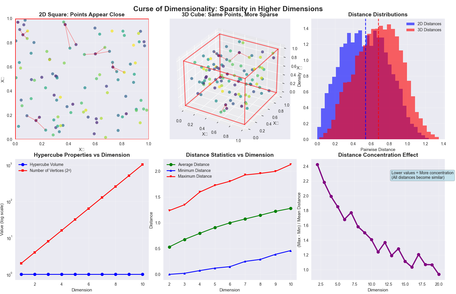
This sparsity has profound consequences for machine learning algorithms, particularly those that rely on distance metrics, such as k-Nearest Neighbors (k-NN). In a high-dimensional space, the distance between any two points can become almost equidistant, rendering concepts of “neighborhood” and “locality” meaningless. For a model, this means that it becomes much harder to find meaningful patterns, as every data point appears as an outlier. The model may learn spurious correlations from the noise inherent in the vast feature space, leading to excellent performance on the training data but a catastrophic failure to generalize to new, unseen data—a classic symptom of overfitting. Feature selection directly mitigates this by reducing \( p \), thereby decreasing the volume of the feature space and increasing the density of the training samples.
Benefits of a Reduced Feature Space
Reducing the number of features offers several tangible benefits in an AI engineering context. The most immediate is the reduction in computational cost. Training a model with fewer features requires less memory and fewer CPU/GPU cycles, leading to faster training times and lower operational costs, especially in cloud environments where resources are metered. This is particularly critical in production systems that require frequent retraining.
Second, a simpler model with fewer features is often more interpretable. When a model relies on hundreds or thousands of variables, it becomes a “black box,” making it difficult for engineers and business stakeholders to understand its decision-making process. A model built on a small, curated set of features is easier to analyze, debug, and trust. This is a crucial requirement in regulated industries like finance and healthcare, where model transparency is mandated.
Finally, and most importantly, feature selection often leads to improved predictive performance. By removing irrelevant and redundant features, we eliminate sources of noise that can confuse the learning algorithm. This allows the model to focus on the true signal within the data, resulting in a lower generalization error and a more robust model that is less sensitive to minor variations in the input data. The goal is to find the “sweet spot” where the feature set is maximally informative without being overly complex, a principle that aligns with Occam’s Razor: the simplest solution is often the best one.
Categories of Feature Selection Methods
Feature selection techniques are broadly classified into three families—filter, wrapper, and embedded methods—based on how they interact with the chosen machine learning model. The choice of method involves a trade-off between computational expense and the potential for achieving optimal model performance.
Filter Methods
Filter methods are the simplest and most computationally efficient category. They operate by assessing the intrinsic properties of the features, typically through univariate statistical tests, and assigning a score to each one. A threshold is then applied to these scores to filter out (i.e., select) the features that are deemed most relevant. The key characteristic of filter methods is that their entire selection process is performed as a preprocessing step, independent of any machine learning algorithm. This makes them very fast and scalable to extremely high-dimensional datasets.
Common statistical measures used in filter methods include:
- Chi-squared (\(\chi^2\)) test: This test is used for categorical features and a categorical target. It measures the dependence between two categorical variables by comparing the observed frequencies in a contingency table to the frequencies that would be expected if the variables were independent. The null hypothesis is that the two variables are independent. A high \(\chi^2\) statistic indicates that the null hypothesis should be rejected, implying a strong association between the feature and the target. The \(\chi^2\) statistic is calculated as:\[ \chi^2 = \sum_{i=1}^{r} \sum_{j=1}^{c} \frac{(O_{ij} – E_{ij})^2}{E_{ij}} \] where \(O_{ij}\) is the observed frequency and \(E_{ij}\) is the expected frequency for the cell in row \(i\) and column \(j\).
- ANOVA F-test: This is used for numerical features and a categorical target. It computes the ratio of the variance between groups to the variance within groups. A large F-value indicates that there is more variation between the groups (defined by the target variable’s categories) than within them, suggesting the feature is a good discriminator.
- Mutual Information: This information-theoretic measure quantifies the dependency between two variables, capturing both linear and non-linear relationships. It measures how much information about one variable is obtained through the other. For two random variables \(X\) and \(Y\), the mutual information \(I(X;Y)\) is given by:\[ I(X;Y) = \sum_{y \in Y} \sum_{x \in X} p(x,y) \log\left(\frac{p(x,y)}{p(x)p(y)}\right) \]A higher mutual information value indicates a stronger relationship.
While fast and effective at removing clearly irrelevant features, filter methods have a significant drawback: they evaluate each feature in isolation (univariately) and ignore feature dependencies. A feature might be useless by itself but highly predictive when combined with another. Filter methods are incapable of detecting such interactions.
graph TD
    subgraph Filter Method Workflow
    direction TB
        A[/"Raw Dataset (n samples, p features)"/];
        B{"Calculate Feature Scores<br><i>(e.g., Chi-squared, Mutual Info)</i>"};
        C["Rank Features by Score"];
        D{"Select Top 'k' Features<br>or Features Above Threshold"};
        E[/"Selected Features (k < p)"/];
        F(("Train ML Model"));

        A --> B;
        B --> C;
        C --> D;
        D --> E;
        E --> F;
    end

    %% Styling
    style A fill:#9b59b6,stroke:#9b59b6,stroke-width:1px,color:#ebf5ee
    style B fill:#78a1bb,stroke:#78a1bb,stroke-width:1px,color:#283044
    style C fill:#78a1bb,stroke:#78a1bb,stroke-width:1px,color:#283044
    style D fill:#f39c12,stroke:#f39c12,stroke-width:1px,color:#283044
    style E fill:#2d7a3d,stroke:#2d7a3d,stroke-width:2px,color:#ebf5ee
    style F fill:#e74c3c,stroke:#e74c3c,stroke-width:1px,color:#ebf5ee
Wrapper Methods
Wrapper methods address the primary limitation of filter methods by using a specific machine learning model to evaluate the utility of feature subsets. The feature selection process “wraps” around the model: a subset of features is selected, the model is trained and evaluated on this subset, and the process is repeated with different subsets. The subset that yields the best model performance (e.g., highest accuracy, lowest error) is chosen.
This approach is inherently more powerful than filter methods because it accounts for feature interactions and dependencies as seen by the model itself. However, this power comes at a significant computational cost. The number of possible feature subsets is \(2^p\), where \(p\) is the number of features. Exhaustively searching this space is computationally infeasible for all but the smallest datasets. Therefore, wrapper methods employ greedy search strategies to navigate the space of feature subsets.
A prominent example is Recursive Feature Elimination (RFE). RFE works as follows:
- Train the chosen model on the initial set of all \(p\) features.
- Calculate a feature importance score for each feature (e.g., using model coefficients or tree-based importance).
- Prune the least important feature.
- Repeat the process with the remaining \(p-1\) features until the desired number of features is reached.
graph TD
    subgraph "Wrapper Method: Recursive Feature Elimination (RFE)"
        Start("Start with all 'p' features");
        TrainModel["Train Model<br><i>(e.g., Logistic Regression)</i>"];
        ScoreFeatures{"Calculate Feature Importance<br><i>(e.g., from coefficients)</i>"};
        PruneFeature["Prune Least Important Feature"];
        CheckCondition{"Desired Number of<br>Features Reached?"};
        End("Output Final Feature Set");

        Start --> TrainModel;
        TrainModel --> ScoreFeatures;
        ScoreFeatures --> PruneFeature;
        PruneFeature --> CheckCondition;
        CheckCondition -- "No" --> TrainModel;
        CheckCondition -- "Yes" --> End;
    end

    %% Styling
    style Start fill:#283044,stroke:#283044,stroke-width:2px,color:#ebf5ee
    style TrainModel fill:#e74c3c,stroke:#e74c3c,stroke-width:1px,color:#ebf5ee
    style ScoreFeatures fill:#78a1bb,stroke:#78a1bb,stroke-width:1px,color:#283044
    style PruneFeature fill:#d63031,stroke:#d63031,stroke-width:1px,color:#ebf5ee
    style CheckCondition fill:#f39c12,stroke:#f39c12,stroke-width:1px,color:#283044
    style End fill:#2d7a3d,stroke:#2d7a3d,stroke-width:2px,color:#ebf5ee
The model is retrained at each step, making RFE computationally intensive. However, it is often very effective at finding a highly predictive and compact feature set. Other wrapper strategies include Sequential Feature Selection (SFS), which can be forward (starting with an empty set and adding features one by one) or backward (starting with all features and removing them one by one).
Note: The choice of model in a wrapper method is crucial. A feature subset that is optimal for a linear model may be suboptimal for a complex, non-linear model like a Gradient Boosting Machine.
Embedded Methods
Embedded methods offer a compromise between the computational efficiency of filter methods and the performance-oriented approach of wrapper methods. In this category, the feature selection process is an intrinsic part of the model training process itself. The algorithm learns which features are most important as it builds the model, making it more efficient than wrapper methods, which require retraining a model for each subset evaluation.
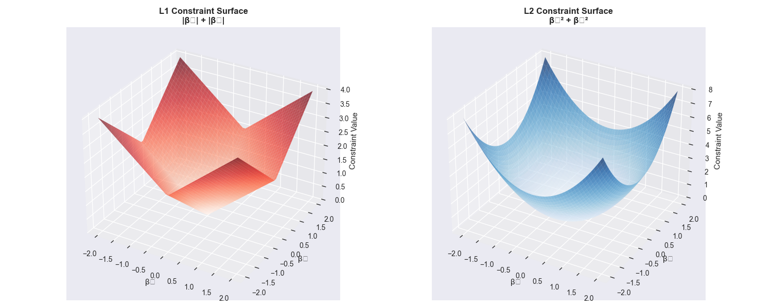
The most well-known examples of embedded methods are those based on L1 (Lasso) regularization. Regularization is a technique used to prevent overfitting by adding a penalty term to the model’s loss function. The L1 penalty term is the sum of the absolute values of the model’s coefficients (weights). The objective function for a linear model with L1 regularization is:\[ \text{minimize} \left( \sum_{i=1}^{n} (y_i – \sum_{j=1}^{p} x_{ij}\beta_j)^2 + \lambda \sum_{j=1}^{p} |\beta_j| \right) \]
Here, the first term is the standard sum of squared errors, and the second is the L1 penalty, controlled by the hyperparameter \(\lambda\). A key property of the L1 penalty is that it can shrink some coefficients \(\beta_j\) to be exactly zero. Features corresponding to zero-valued coefficients are effectively removed from the model. By tuning \(\lambda\), we can control the sparsity of the model, and thus, the number of selected features.

Another powerful class of embedded methods comes from tree-based models, such as Random Forests and Gradient Boosting Machines. These models naturally compute feature importance scores during training. For a decision tree, the importance of a feature is typically calculated as the total reduction in impurity (e.g., Gini impurity or entropy) brought about by splits on that feature, averaged across all trees in the ensemble. Features with high importance scores are considered more relevant to the prediction task. By training a tree-based model and then selecting features based on a certain importance threshold, we are performing embedded feature selection. This approach is computationally efficient and can capture complex, non-linear feature interactions.
| Method Type | Core Idea | Pros | Cons | Common Algorithms |
|---|---|---|---|---|
| Filter | Selects features based on their intrinsic statistical properties, independent of any ML model. | – Very fast and computationally inexpensive. – Scalable to high-dimensional data. – Avoids overfitting. |
– Ignores feature dependencies and interactions. – May select redundant features. – Not optimized for a specific model. |
Chi-squared Test, ANOVA F-test, Mutual Information, Correlation Coefficient |
| Wrapper | Uses a specific ML model to evaluate the utility of different feature subsets. The selection is “wrapped” around the model. | – Considers feature interactions. – Optimized for the chosen model’s performance. – Often results in better predictive accuracy. |
– Computationally very expensive. – High risk of overfitting to the training data. – Infeasible for very large feature sets. |
Recursive Feature Elimination (RFE), Sequential Feature Selection (SFS), Genetic Algorithms |
| Embedded | Feature selection is an integral, built-in part of the model training process itself. | – More efficient than wrapper methods. – Considers feature interactions. – Less prone to overfitting than wrappers. |
– Tied to a specific model class. – The selected features are specific to the chosen algorithm. |
L1 (Lasso) Regularization, Tree-based Importance (Random Forest, GBM), Elastic Net |
Practical Examples and Implementation
Theoretical understanding of feature selection methods is essential, but true mastery comes from practical application. This section translates the concepts of filter, wrapper, and embedded methods into executable Python code using the powerful scikit-learn library. We will use a synthetic classification dataset to provide clear, reproducible examples of how to implement, visualize, and interpret the results of each technique.
Tip: For all implementations, it is critical to split your data into training and testing sets before applying any feature selection. Feature selection methods should be “fit” only on the training data to prevent data leakage from the test set, which would lead to an overly optimistic evaluation of model performance.
# Common setup for all examples
import numpy as np
import pandas as pd
import matplotlib.pyplot as plt
import seaborn as sns
from sklearn.model_selection import train_test_split
from sklearn.preprocessing import MinMaxScaler
from sklearn.datasets import make_classification

# Generate a synthetic dataset
# 1000 samples, 25 features, 15 informative, 5 redundant, 5 noisy
X, y = make_classification(n_samples=1000, n_features=25, n_informative=15,
                           n_redundant=5, n_repeated=0, n_classes=2,
                           n_clusters_per_class=2, flip_y=0.01,
                           class_sep=0.8, random_state=42)

# Convert to DataFrame for easier handling
feature_names = [f'feature_{i}' for i in range(X.shape[1])]
X = pd.DataFrame(X, columns=feature_names)

# Split data into training and testing sets
X_train, X_test, y_train, y_test = train_test_split(X, y, test_size=0.2, random_state=42, stratify=y)

# Scale features (important for many models and some selection methods)
# Note: Chi-squared requires non-negative features.
scaler = MinMaxScaler()
X_train_scaled = scaler.fit_transform(X_train)
X_test_scaled = scaler.transform(X_test)
X_train_scaled = pd.DataFrame(X_train_scaled, columns=feature_names)
Mathematical Concept Implementation: Filter Methods
Filter methods use statistical tests to score and rank features. Here, we implement two common methods using scikit-learn‘s SelectKBest, which allows us to select a fixed number (k) of the highest-scoring features.
Chi-Squared (\(\chi^2\)) Implementation
The Chi-squared test is suitable for categorical features. Since our data is numerical, we use MinMaxScaler to ensure all values are non-negative, a prerequisite for this test in scikit-learn.
from sklearn.feature_selection import SelectKBest, chi2

# We want to select the top 15 features
k_best_chi2 = SelectKBest(score_func=chi2, k=15)

# Fit on the scaled training data
k_best_chi2.fit(X_train_scaled, y_train)

# Get scores and selected feature names
chi2_scores = pd.DataFrame({'Feature': X_train.columns, 'Score': k_best_chi2.scores_})
chi2_scores = chi2_scores.sort_values(by='Score', ascending=False)
selected_features_chi2 = chi2_scores.head(15)['Feature'].tolist()

print("Top 15 features selected by Chi-squared:")
print(selected_features_chi2)

# Visualization of scores
plt.figure(figsize=(12, 8))
sns.barplot(x='Score', y='Feature', data=chi2_scores.head(20), palette='viridis')
plt.title('Top 20 Feature Scores using Chi-Squared Test')
plt.xlabel('Chi-Squared Score')
plt.ylabel('Feature')
plt.tight_layout()
plt.show()
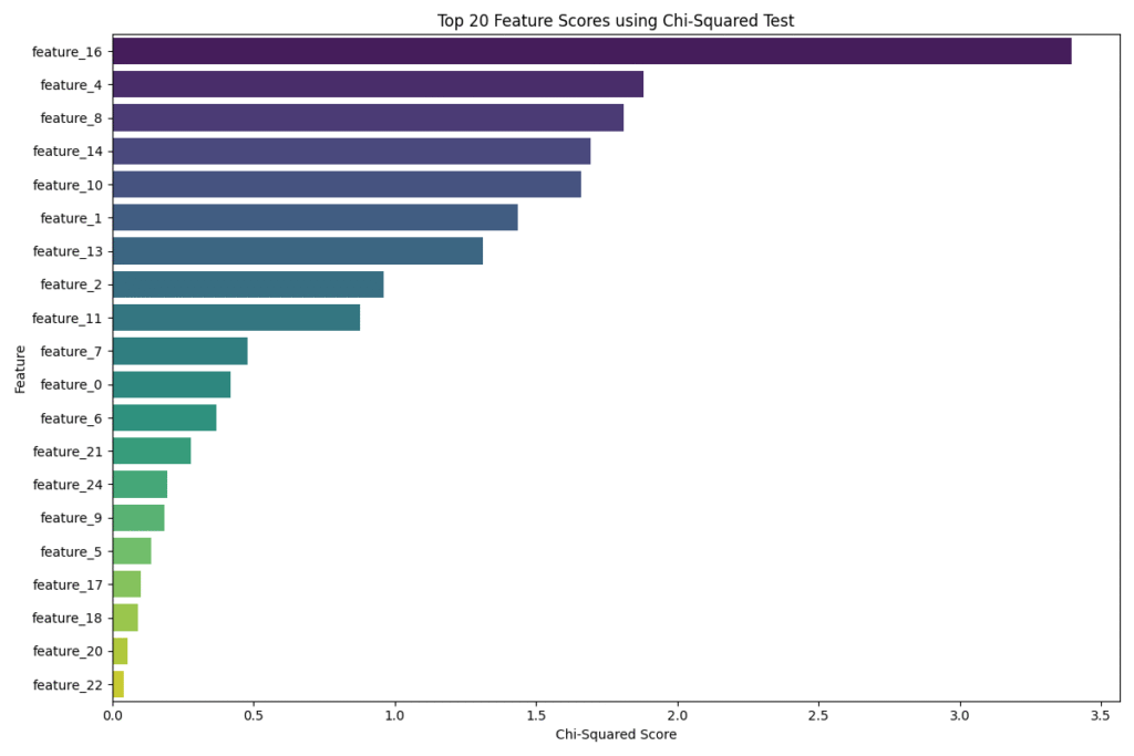
This code first applies the chi2 test to all features and then selects the 15 with the highest scores. The bar plot provides a clear visual ranking, allowing us to see the relative importance of each feature according to this statistical measure. The selected features are those that show the strongest statistical dependence on the target variable.
AI/ML Application Examples: Wrapper and Embedded Methods
Unlike filter methods, wrapper and embedded methods leverage a machine learning model to guide the selection process. This makes them more computationally intensive but often more effective at finding feature subsets that are optimized for a specific algorithm.
Recursive Feature Elimination (RFE) Implementation
RFE is a classic wrapper method. We will use a LogisticRegression model as the estimator to guide the elimination process. RFE will iteratively train the model, discard the least important feature (based on the model’s coefficients), and repeat until the desired number of features remains.
# Common setup for all examples
import numpy as np
import matplotlib.pyplot as plt
import seaborn as sns
from sklearn.model_selection import train_test_split
from sklearn.preprocessing import MinMaxScaler
from sklearn.datasets import make_classification
from sklearn.feature_selection import RFE
from sklearn.linear_model import LogisticRegression
import pandas as pd


# Generate a synthetic dataset
# 1000 samples, 25 features, 15 informative, 5 redundant, 5 noisy
X, y = make_classification(n_samples=1000, n_features=25, n_informative=15,
                           n_redundant=5, n_repeated=0, n_classes=2,
                           n_clusters_per_class=2, flip_y=0.01,
                           class_sep=0.8, random_state=42)

# Convert to DataFrame for easier handling
feature_names = [f'feature_{i}' for i in range(X.shape[1])]
X = pd.DataFrame(X, columns=feature_names)

# Split data into training and testing sets
X_train, X_test, y_train, y_test = train_test_split(X, y, test_size=0.2, random_state=42, stratify=y)

# Scale features (important for many models and some selection methods)
# Note: Chi-squared requires non-negative features.
scaler = MinMaxScaler()
X_train_scaled = scaler.fit_transform(X_train)
X_test_scaled = scaler.transform(X_test)
X_train_scaled = pd.DataFrame(X_train_scaled, columns=feature_names)

# Initialize the model and RFE
# We want to select 15 features
estimator = LogisticRegression(max_iter=1000, random_state=42)
selector_rfe = RFE(estimator, n_features_to_select=15, step=1)

# Fit RFE on the training data
selector_rfe = selector_rfe.fit(X_train_scaled, y_train)

# Get the selected features
selected_features_rfe = X_train.columns[selector_rfe.support_].tolist()

print("Features selected by RFE:")
print(selected_features_rfe)

# Check the ranking of features
rfe_ranking = pd.DataFrame({'Feature': X_train.columns, 'Rank': selector_rfe.ranking_})
print("\nFeature Ranking from RFE:")
print(rfe_ranking.sort_values(by='Rank'))
Outputs:
Features selected by RFE:
['feature_1', 'feature_2', 'feature_4', 'feature_5', 'feature_6', 'feature_7', 'feature_8', 'feature_10', 'feature_11', 'feature_13', 'feature_14', 'feature_15', 'feature_16', 'feature_18', 'feature_21']

Feature Ranking from RFE:
       Feature  Rank
11  feature_11     1
1    feature_1     1
2    feature_2     1
18  feature_18     1
4    feature_4     1
5    feature_5     1
6    feature_6     1
7    feature_7     1
8    feature_8     1
10  feature_10     1
21  feature_21     1
16  feature_16     1
13  feature_13     1
14  feature_14     1
15  feature_15     1
17  feature_17     2
22  feature_22     3
24  feature_24     4
23  feature_23     5
3    feature_3     6
19  feature_19     7
9    feature_9     8
20  feature_20     9
0    feature_0    10
12  feature_12    11
The selector_rfe.support_ attribute returns a boolean mask indicating which features were selected. The ranking_ attribute shows the elimination order, with a rank of 1 indicating the best features. RFE directly optimizes for the feature set that works best with the chosen estimator, in this case, LogisticRegression.
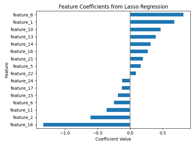
Embedded Method: L1 (Lasso) Regularization
Lasso regression is a powerful embedded method that performs feature selection by shrinking the coefficients of less important features to exactly zero. We use LassoCV to find the optimal regularization strength alpha (equivalent to \(\lambda\) in our formula) via cross-validation.
from sklearn.linear_model import LassoCV
from sklearn.metrics import mean_squared_error

# LassoCV for regression tasks, so we use it here for demonstration
# In a classification context, one would use LogisticRegression with 'l1' penalty
lasso = LassoCV(cv=5, random_state=42, max_iter=10000).fit(X_train_scaled, y_train)

# Get the coefficients
lasso_coefs = pd.DataFrame({'Feature': X_train.columns, 'Coefficient': lasso.coef_})
selected_features_lasso = lasso_coefs[lasso_coefs['Coefficient'] != 0]['Feature'].tolist()

print(f"Optimal alpha (lambda) found by LassoCV: {lasso.alpha_}")
print(f"Number of features selected by Lasso: {len(selected_features_lasso)}")
print("Selected features:")
print(selected_features_lasso)

# Visualize coefficients
plt.figure(figsize=(12, 8))
lasso_coefs[lasso_coefs['Coefficient'] != 0].sort_values('Coefficient').plot(kind='barh', x='Feature', y='Coefficient', legend=False)
plt.title('Feature Coefficients from Lasso Regression')
plt.xlabel('Coefficient Value')
plt.axvline(x=0, color='.5')
plt.tight_layout()
plt.show()
Embedded Method: Tree-Based Feature Importance
Tree-based ensembles like Random Forest naturally calculate feature importance. We can train a RandomForestClassifier and use its feature_importances_ attribute to select features.
from sklearn.ensemble import RandomForestClassifier
from sklearn.feature_selection import SelectFromModel

# Train a Random Forest model
rf = RandomForestClassifier(n_estimators=100, random_state=42, n_jobs=-1)
rf.fit(X_train_scaled, y_train)

# Get feature importances
importances = pd.DataFrame({'Feature': X_train.columns, 'Importance': rf.feature_importances_})
importances = importances.sort_values(by='Importance', ascending=False)

# Select features using SelectFromModel
# The threshold can be a value like 'median' or a specific float
selector_sfm = SelectFromModel(rf, threshold='median', prefit=True)
selected_features_sfm = X_train.columns[selector_sfm.get_support()].tolist()

print(f"Number of features selected by Random Forest Importance: {len(selected_features_sfm)}")
print("Selected features:")
print(selected_features_sfm)

# Visualize feature importances
plt.figure(figsize=(12, 8))
sns.barplot(x='Importance', y='Feature', data=importances.head(15), palette='plasma')
plt.title('Top 15 Feature Importances from Random Forest')
plt.xlabel('Importance Score')
plt.ylabel('Feature')
plt.tight_layout()
plt.show()
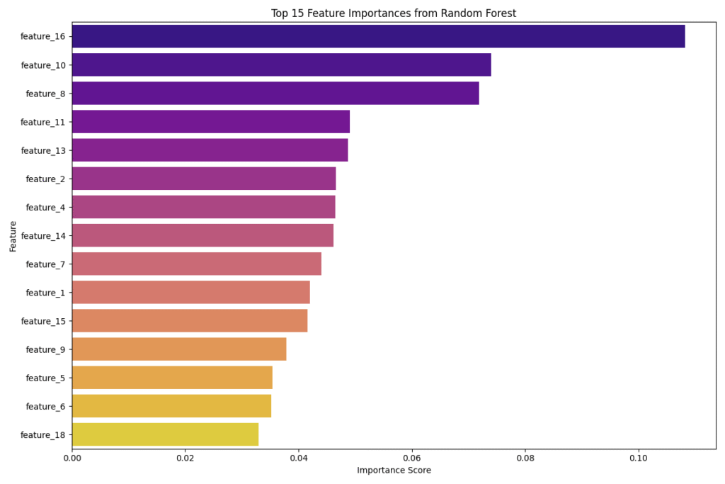
This approach is highly effective as it captures non-linear relationships and feature interactions. The bar plot clearly shows which features the Random Forest model found most predictive. SelectFromModel provides a convenient way to perform the selection based on these importance scores.
Real-World Problem Applications
These techniques are not just academic exercises; they are fundamental to solving real-world problems.
- In Medical Diagnosis: A dataset of patient information might contain hundreds of biomarkers (features). Using RFE with a Support Vector Machine could identify the 10-15 most critical biomarkers for predicting the presence of a disease, leading to cheaper, faster, and more targeted diagnostic tests.
- In Customer Churn Prediction: A telecom company might have thousands of features describing customer behavior. Using Lasso regression, a company can identify the key drivers of churn (e.g., number of support calls, plan type, contract length). The resulting sparse model is not only predictive but also highly interpretable, providing actionable insights for the business to create targeted retention campaigns.
- In Image Recognition: While deep learning models perform end-to-end feature learning, traditional computer vision pipelines often rely on handcrafted features like SIFT or HOG. In a dataset of thousands of such features, a filter method like Mutual Information could be used to quickly pre-select the most promising features before feeding them into a classifier, drastically reducing training time.
Industry Applications and Case Studies
The principles of feature selection are actively applied across numerous industries to build more efficient and effective AI systems. These applications demonstrate the tangible business value derived from moving beyond raw data to curated, informative feature sets.
- Financial Services: Credit Risk Modeling and Fraud Detection
- Use Case: A bank developing a model to predict loan defaults has access to hundreds of applicant attributes, from credit history and income to behavioral data.
- Technical Implementation: L1 (Lasso) regularization is widely used in this domain. Its ability to produce a sparse model is highly valued not only for performance but also for regulatory compliance. Regulators often require financial models to be interpretable. By zeroing out the coefficients of less impactful features, Lasso creates a simpler, more auditable model that highlights the key factors driving credit risk. For real-time fraud detection, filter methods are used to quickly screen thousands of transaction features, passing only the most relevant subset to a more complex downstream model, thus meeting low-latency requirements.
- Business Impact: Improved model accuracy leads to fewer defaults and reduced financial losses. The enhanced interpretability satisfies regulatory demands and builds trust in the system. Faster fraud detection models can prevent fraudulent transactions in real-time, saving millions.
- Healthcare and Bioinformatics: Genomic Data Analysis
- Use Case: In cancer research, scientists analyze microarray data which can contain measurements for tens of thousands of genes (features) for a relatively small number of patients. The goal is to identify the specific genes that are most indicative of a particular type of cancer.
- Technical Implementation: This is a classic “high-dimensional” problem (\(p \gg n\)). Wrapper methods like Recursive Feature Elimination with Cross-Validation (RFECV) are often employed. RFECV systematically tests feature subsets of different sizes, using cross-validation to find the optimal number of genes that yields the best predictive performance for a classifier like an SVM. This helps in identifying a small, stable set of genetic biomarkers.
- Business Impact: Identifying key biomarkers can lead to the development of new diagnostic tests, personalized medicine, and targeted drug therapies, representing a massive return on investment and a significant advancement in patient care.
- E-commerce and Marketing: Customer Segmentation and Personalization
- Use Case: An online retailer wants to personalize marketing campaigns by understanding which customer attributes are most predictive of purchasing behavior. They have access to vast amounts of data, including browsing history, demographics, past purchases, and interaction with previous campaigns.
- Technical Implementation: Tree-based embedded methods, particularly feature importance from Gradient Boosting Machines (GBMs), are extremely popular. A GBM can be trained on the full feature set to predict a customer’s likelihood to purchase. The resulting feature importance scores, which capture complex non-linear interactions, are then used to select the top drivers of engagement.
- Business Impact: By focusing marketing efforts on the most influential features (e.g., “time spent on product page,” “items in cart”), the company can create highly effective, personalized campaigns. This leads to higher conversion rates, increased customer loyalty, and a more efficient allocation of the marketing budget.
Best Practices and Common Pitfalls
Effectively integrating feature selection into an AI development workflow requires more than just knowing the algorithms; it demands a strategic approach and an awareness of potential traps. Adhering to best practices ensures that the process yields genuine performance improvements and robust, reliable models.
- Prevent Data Leakage at All Costs: This is the most critical rule. Feature selection, like any other preprocessing step (e.g., scaling, imputation), must be learned only from the training portion of your data. If you use the entire dataset to select features and then perform a train-test split, information from the test set has “leaked” into your feature selection process. This will make your model’s performance on the test set appear artificially high. The correct workflow is always: 1) Split data into training and validation/test sets. 2) Fit your feature selection method on the training data only. 3) Transform both the training and test sets using the fitted selector.Warning: Performing feature selection before splitting your data is one of the most common and serious mistakes in applied machine learning. Always use pipelines (e.g.,
sklearn.pipeline.Pipeline) to encapsulate your preprocessing and modeling steps, which helps enforce this correct workflow. - Understand the Bias of Your Selection Method: Each feature selection method has its own inherent biases. Univariate filter methods are biased towards features that are predictive on their own, potentially discarding features that are only useful in combination with others. RFE is biased by the model you choose to guide it; a linear model will prefer linearly related features. Tree-based methods are good at finding non-linear interactions but can sometimes overstate the importance of high-cardinality numerical features. It is often wise to try multiple feature selection methods and compare the resulting feature sets and model performances.
- Don’t Conflate Feature Importance with Causal Inference: A high feature importance score indicates that a feature is predictive for your model, not necessarily that it has a causal relationship with the target. For example, in a dataset predicting house prices, the “number of bathrooms” might have a high importance score. This doesn’t mean adding a bathroom causes the price to increase; rather, it’s strongly correlated with other factors like square footage that are the true causal drivers. Be precise in your interpretation and communication with stakeholders.
- Consider Feature Redundancy and Multicollinearity: Some methods, especially univariate filters, might select multiple features that are highly correlated with each other (e.g., “height in feet” and “height in inches”). While these features may all be individually predictive, their inclusion together can make models like linear regression unstable. After an initial selection, it can be beneficial to analyze the correlation matrix of the selected features and consider removing redundant ones to create a more parsimonious and robust model.
- Tune the Number of Features as a Hyperparameter: How many features should you select? 10? 50? 100? This number is effectively a hyperparameter of your entire modeling pipeline. Instead of picking an arbitrary number, you should tune it. Techniques like
RFECVin scikit-learn perform recursive feature elimination with built-in cross-validation to automatically determine the optimal number of features that maximizes model performance.
Hands-on Exercises
These exercises are designed to solidify your understanding of feature selection by applying the concepts to practical problems. They progress from foundational application to more complex, comparative analysis.
- Exercise 1: Univariate Filter Selection on a Real Dataset
- Objective: Apply and compare two different univariate filter methods on a real-world dataset.
- Task:
- Load the Breast Cancer Wisconsin dataset from
sklearn.datasets. - Perform a train-test split.
- Use
SelectKBestto select the top 10 features using two different scoring functions:f_classif(ANOVA F-test) andmutual_info_classif. - Train a
LogisticRegressionmodel on the 10 features selected by each method. - Compare the performance (e.g., accuracy, F1-score) of the two models on the test set. Did the choice of scoring function make a difference?
- Load the Breast Cancer Wisconsin dataset from
- Success Criteria: You have successfully trained and evaluated two models, each with a different feature subset, and can articulate the performance differences.
- Exercise 2: Finding the Optimal Number of Features with RFECV
- Objective: Use Recursive Feature Elimination with Cross-Validation (RFECV) to automatically determine the optimal number of features.
- Task:
- Use the same Breast Cancer dataset and train-test split from Exercise 1.
- Initialize an
SVC(Support Vector Classifier) with alinearkernel. - Use
sklearn.feature_selection.RFECVwith the SVC estimator to perform feature selection on the training data. Usef1as the scoring metric for cross-validation. - Plot the cross-validation scores against the number of features selected.
- Identify the optimal number of features found by
RFECV. Train a final SVC model using only these optimal features and evaluate it on the test set.
- Success Criteria: You have produced a plot showing performance vs. number of features and have trained a final model using the optimal feature set identified by the RFECV process.
- Exercise 3: Comparative Analysis of Selection Methods (Team Activity)
- Objective: Conduct a comprehensive comparison of filter, wrapper, and embedded methods for a regression problem.
- Task:
- Load the California Housing dataset from
sklearn.datasets. - Perform a train-test split and scale the features.
- Team Member A (Filter): Use
SelectKBestwithf_regressionto select the top 5 features. - Team Member B (Wrapper): Use
RFEwith aLinearRegressionmodel to select the top 5 features. - Team Member C (Embedded): Use
LassoCVto perform feature selection. Identify the features with non-zero coefficients. - As a team, train a
RandomForestRegressormodel on each of the selected feature subsets. Also, train a baseline model on all features. - Compare the Mean Squared Error (MSE) of all models on the test set. Discuss the trade-offs (performance vs. complexity vs. computation time) of each feature selection approach.
- Load the California Housing dataset from
- Success Criteria: The team produces a comparative report or presentation summarizing the results, including the feature sets chosen by each method and the final model performance metrics.
Tools and Technologies
The modern AI/ML ecosystem provides a rich set of tools for performing feature selection, primarily within the Python scientific computing stack.
- scikit-learn: This is the cornerstone library for feature selection in Python. Its
sklearn.feature_selectionmodule is comprehensive, offering implementations of nearly all the methods discussed in this chapter, includingSelectKBestfor filter methods,RFEandRFECVfor wrapper methods, andSelectFromModelfor applying embedded method results. Its seamless integration with other components likePipelineandGridSearchCVmakes it indispensable for building robust MLOps workflows. - pandas & NumPy: These libraries are fundamental for data manipulation.
pandasDataFrames are used to hold the data and feature names, making it easy to track which features are selected.NumPyprovides the underlying efficient array structures thatscikit-learnrelies on. - Statsmodels: For engineers who require deeper statistical insight, the
statsmodelslibrary offers more detailed statistical tests and results thanscikit-learn, including p-values and confidence intervals for model coefficients, which can be useful for certain types of feature analysis. - Specialized Libraries: For more advanced or specific use cases, several third-party libraries exist.
feature-engine: This library provides a wide array of feature engineering and selection transformers that are designed to be fully compatible with scikit-learn pipelines.boruta_py: An implementation of the Boruta feature selection algorithm, which is a clever wrapper method based on Random Forests that is particularly effective at finding all relevant features in a dataset.
- MLOps Platforms (MLflow, Kubeflow): In a production environment, feature selection is not a one-off task. MLOps platforms like MLflow can be used to track experiments with different feature subsets, log the selected features as artifacts, and version control the entire pipeline, ensuring reproducibility and governance.
Summary
This chapter has provided a comprehensive exploration of feature selection, a critical process for building efficient, interpretable, and high-performing machine learning models.
- Key Concepts: We established the motivation for feature selection, primarily to combat the curse of dimensionality, reduce model complexity, decrease computational cost, and improve generalization performance.
- Core Techniques: We dissected the three main families of feature selection methods:
- Filter Methods: Fast and scalable, using statistical tests independent of the ML model (e.g., Chi-squared, ANOVA).
- Wrapper Methods: Model-centric and powerful, using a specific model to evaluate feature subsets (e.g., Recursive Feature Elimination).
- Embedded Methods: An efficient hybrid where selection is integrated into model training (e.g., L1/Lasso Regularization, tree-based importance).
- Practical Skills: You have gained hands-on experience implementing these techniques in Python with
scikit-learn, learning how to apply them correctly within a proper validation framework to avoid data leakage. - Real-World Applicability: The ability to curate an optimal feature set is a highly sought-after skill in AI engineering, directly impacting business outcomes in fields from finance to healthcare. Mastering feature selection moves you from being a model user to a model builder who can engineer solutions that are not only predictive but also practical for production deployment.
Further Reading and Resources
- Scikit-learn Documentation: The official documentation for the
sklearn.feature_selectionmodule is the definitive resource for implementation details and examples. https://scikit-learn.org/stable/modules/feature_selection.html - “An Introduction to Statistical Learning” by James, Witten, Hastie, and Tibshirani: Chapter 6 provides an excellent and accessible theoretical background on feature selection, particularly subset selection and regularization methods like Lasso.
- “Regularization Paths for Generalized Linear Models via Coordinate Descent” by Friedman, Hastie, and Tibshirani (2010): The seminal research paper detailing the highly efficient algorithm behind Lasso and Elastic Net implementations in libraries like scikit-learn.
- “Boruta – A System for Feature Selection” by M. B. Kursa and W. R. Rudnicki: The original paper on the Boruta algorithm, for those interested in advanced wrapper methods.
- Kaggle Notebooks and Competitions: Many high-ranking Kaggle solutions include sophisticated feature selection pipelines. Exploring these provides practical insight into what works on complex, real-world datasets.
- “Feature Engineering for Machine Learning” by Alice Zheng & Amanda Casari: A practical guide that covers feature selection as a key part of the broader feature engineering process.
Glossary of Terms
- Curse of Dimensionality: A term describing various phenomena that arise when analyzing data in high-dimensional spaces, such as data sparsity, which makes it difficult for algorithms to find meaningful patterns.
- Data Leakage: The introduction of information from outside the training dataset into the model building process, often leading to overly optimistic performance estimates. In feature selection, this occurs if the test set is used to inform which features are chosen.
- Embedded Method: A category of feature selection techniques where the selection process is an integral part of the model training algorithm (e.g., Lasso regression).
- Filter Method: A category of feature selection techniques where features are scored and selected based on their intrinsic statistical properties, independent of any machine learning model.
- L1 Regularization (Lasso): A regularization technique that adds a penalty equal to the sum of the absolute values of the coefficients to the loss function. It has the property of shrinking some coefficients to exactly zero, thus performing feature selection.
- Mutual Information: A measure from information theory that quantifies the statistical dependency between two random variables, capturing both linear and non-linear relationships.
- Recursive Feature Elimination (RFE): A wrapper method for feature selection that recursively trains a model, considers the least important feature, removes it, and repeats the process on the remaining set of features.
- Univariate Selection: A feature selection strategy that analyzes each feature individually to determine the strength of its relationship with the target variable.
- Wrapper Method: A category of feature selection techniques that uses a specific machine learning model to evaluate the utility of different subsets of features.
