
Chapter 31: Feature Engineering: Creating New Features from Raw Data
Chapter Objectives
Upon completing this chapter, you will be able to:
- Understand the fundamental role of feature engineering in the machine learning lifecycle and its impact on model performance, interpretability, and robustness.
- Implement core feature creation techniques, including polynomial features and interaction terms, using industry-standard libraries like scikit-learn and pandas.
- Design and apply domain-specific features for various data types, with a focus on creating temporal features from time-series data.
- Analyze the trade-offs between feature complexity, model performance, and the risk of overfitting, such as the curse of dimensionality.
- Develop systematic and reproducible feature engineering pipelines using tools like scikit-learn’s
PipelineandColumnTransformerfor production environments. - Integrate feature engineering logic into a larger MLOps workflow, ensuring consistency between training and inference to prevent data leakage.
Introduction
In the landscape of artificial intelligence and machine learning, data is often cited as the new oil. While this analogy highlights its value, it is incomplete. Raw data, like crude oil, is rarely useful in its natural state. It must be refined, processed, and transformed into a valuable commodity. This process of refinement in machine learning is known as feature engineering. It is the critical, often labor-intensive, process of using domain knowledge to extract and create new, informative variables—or “features”—from raw data to facilitate the machine learning process. A well-crafted feature can be the difference between a mediocre model and a state-of-the-art predictive system. It is where data science meets creativity, intuition, and deep subject-matter expertise.
This chapter delves into the art and science of creating new features. We move beyond the preprocessing steps of cleaning and scaling, which were covered in previous chapters, and into the proactive construction of variables that explicitly expose the underlying patterns in the data to our learning algorithms. For instance, a linear model may fail to capture a non-linear trend in housing prices, but by providing it with a feature representing the square footage squared, we give it the tool it needs to model that curvature. Similarly, in retail, raw timestamps are just numbers; engineered features like “day of the week” or “time since last purchase” provide actionable context. This chapter will provide you with a systematic framework for these transformations, covering polynomial and interaction features, domain-specific techniques for temporal and other data types, and the practical implementation of these methods in robust, production-ready pipelines. By mastering feature engineering, you transition from a user of machine learning algorithms to an architect of intelligent systems.
Technical Background
The Philosophy and Importance of Feature Engineering
Beyond Raw Data: Why Models Need Engineered Features
Machine learning models, despite their increasing complexity, do not possess human-like intuition or common-sense understanding of the world. They learn by identifying statistical patterns in the numerical data they are given. The way this data is presented to the model profoundly influences its ability to learn. Feature engineering is the bridge between raw, often uninformative data and the structured, meaningful inputs that algorithms require to build powerful predictive models. Its primary goal is to translate domain knowledge and implicit data relationships into explicit numerical features, thereby making the underlying patterns more accessible to the learning algorithm.
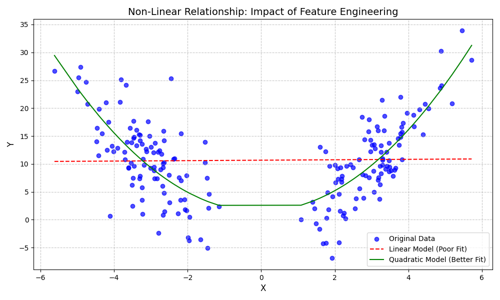
Consider a simple linear regression model. By definition, it can only capture linear relationships between variables. If the true relationship between an input variable \(x\) and the target \(y\) is quadratic (e.g., \(y \approx x^2\)), the model will perform poorly. However, if we engineer a new feature, \(x_{new} = x^2\), and provide both \(x\) and \(x_{new}\) to the model, it can now perfectly capture this relationship by learning a linear equation in the new feature space: \(y = \beta_0 + \beta_1x + \beta_2x_{new}\). We have not changed the model; we have changed the data to better suit the model’s capabilities. This principle applies across all model types. Even complex models like Gradient Boosting Machines and Neural Networks benefit significantly from well-engineered features, as it reduces the burden on the model to learn complex relationships from scratch, often leading to faster training, better performance, and solutions that are more robust and generalizable.
Note: The famous computer scientist Pedro Domingos stated, “some machine learning projects succeed and some fail. What makes the difference? Easily the most important factor is the features used.” This underscores the central role of feature engineering in practical, real-world machine learning applications.
The Art and Science of Feature Creation
Feature engineering is a discipline that blends systematic, scientific methods with creative, artistic intuition derived from domain expertise. The “science” aspect involves applying well-defined transformations that have proven effective across various problems. Techniques like creating polynomial features, interaction terms, or deriving time-based components from a timestamp are standard, reproducible methods. These can often be automated and form the backbone of a feature engineering pipeline. The mathematical foundations for these techniques are clear, and their effect on specific model families can be predicted with a high degree of certainty. For example, adding interaction terms allows tree-based models to learn certain relationships with shallower, more stable trees.
The “art” of feature engineering, however, comes from a deep understanding of the problem domain. It is the ability to hypothesize which feature combinations or transformations might capture a meaningful signal relevant to the business problem. For example, in fraud detection, a data scientist might hypothesize that transactions occurring far from a user’s typical location late at night are suspicious. This leads to engineering features like “distance from home” and “hour of the day.” In e-commerce, one might create a feature for “ratio of items added to cart vs. items purchased” as an indicator of user indecisiveness. These features are not derived from a standard formula but from a creative thought process that connects the data to real-world behaviors. This creative process is often iterative: an engineer proposes a feature, builds it, tests its impact on the model, and refines it. This iterative loop of hypothesis, creation, and evaluation is where the most impactful and novel features are often discovered, providing a significant competitive advantage.
Comparison of Feature Creation Techniques
| Technique | Description | Primary Use Case | Pros & Cons |
|---|---|---|---|
| Polynomial Features | Creating new features by raising existing features to a power (e.g., x², x³). | Capturing non-linear relationships in the data, primarily for linear models. |
+ Allows linear models to fit complex, curved patterns. + Simple to implement and interpret the transformation. – High risk of overfitting, especially with high degrees. – Can lead to a large number of features (curse of dimensionality). |
| Interaction Terms | Creating new features by multiplying two or more existing features (e.g., x₁ * x₂). | Modeling synergistic or antagonistic effects where the impact of one feature depends on another. |
+ Explicitly captures relationships that some models miss. + Can improve model performance and provide deeper insights. – Combinatorial explosion of features if not done selectively. – Requires domain knowledge to create meaningful interactions. |
| Temporal Features | Decomposing timestamps into cyclical or duration-based components. | Revealing time-based patterns in time-series data for forecasting or behavioral analysis. |
+ Unlocks powerful predictive signals from raw timestamps. + Highly effective for seasonality, trends, and event-based modeling. – Requires careful handling of time zones and cyclical encodings. – Can be computationally intensive (e.g., complex rolling windows). |
Foundational Feature Creation Techniques
Polynomial Features: Capturing Non-Linear Relationships
Many real-world phenomena do not follow simple linear patterns. The relationship between advertising spend and sales might exhibit diminishing returns, or the performance of an engine might peak at a certain temperature before declining. Linear models, in their basic form, are incapable of capturing these curved, or non-linear, relationships. Polynomial feature engineering is a powerful technique that extends the capability of linear models (and other models) to handle such data. The core idea is to create new features by raising existing features to a power. For a single feature \(x\), we can create new features \(x^2, x^3, x^4, \dots\).
When these new features are added to the dataset, a linear model can learn a coefficient for each one. For instance, a linear regression model’s equation can be expanded from \(y = \beta_0 + \beta_1x_1\) to a polynomial form like \(y = \beta_0 + \beta_1x_1 + \beta_2x_1^2\). Although the equation is now a quadratic function of the original feature \(x_1\), it remains a linear function of the coefficients \(\beta_0, \beta_1, \beta_2\). This means we can still use the same efficient algorithms to solve for the coefficients as we do for simple linear regression. We have effectively transformed the problem into a higher-dimensional space where the relationship becomes linear.
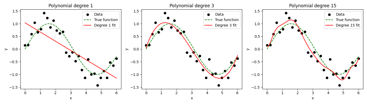
However, this power comes with a significant risk: overfitting. As the degree of the polynomial increases, the model becomes more flexible and can fit the training data more closely. A very high-degree polynomial can weave a curve that passes through every single training data point, achieving near-perfect accuracy on that data. This apparent success is misleading, as the model will have learned the noise in the training data, not the underlying signal. When presented with new, unseen data, its performance will be poor because it has failed to generalize. The trade-off between model complexity and generalizability is a central theme in machine learning, and it is particularly pronounced when using polynomial features. It is crucial to use techniques like cross-validation to select an appropriate polynomial degree and regularization (e.g., Ridge or Lasso regression) to penalize large coefficients and keep the model’s complexity in check.
Interaction Terms: Modeling Feature Synergies
In many systems, the effect of one feature on the outcome depends on the value of another feature. This synergistic or antagonistic relationship is known as an interaction effect. For example, the effectiveness of a digital advertisement might depend on both the ad’s creative content and the time of day it is shown. An ad for coffee might be highly effective in the morning but have little impact in the evening. The features “ad_creative” and “time_of_day” interact. A model that only considers these features independently will miss this crucial context. It might learn an average effect for the coffee ad and an average effect for the morning time slot, but it cannot learn that the combination of the two is particularly powerful.
Interaction terms are new features created by multiplying two or more original features. If we have features \(x_1\) and \(x_2\), their interaction term is \(x_{interaction} = x_1 \times x_2\). By adding this new feature to our dataset, we allow the model to learn a specific coefficient for this combination. The model’s equation could become \(y = \beta_0 + \beta_1x_1 + \beta_2x_2 + \beta_3(x_1x_2)\). The coefficient \(\beta_3\) explicitly captures the interaction effect. A positive \(\beta_3\) would mean that the features have a synergistic effect (the whole is greater than the sum of its parts), while a negative \(\beta_3\) would indicate an antagonistic effect.
This technique is particularly important for linear models and other models that do not capture feature interactions automatically. While tree-based models like Random Forests and Gradient Boosting can implicitly learn interactions through their hierarchical splitting structure, providing explicit interaction terms can still be beneficial. It can allow the model to capture a strong interaction effect with a single split on the new feature, rather than requiring a complex series of splits on the original features. This can lead to simpler, more stable, and sometimes more performant models. The key challenge, as with polynomial features, is combinatorial explosion. For a dataset with \(n\) features, the number of possible pairwise interactions is \(\frac{n(n-1)}{2}\). Creating all possible interactions can lead to a massive feature space, increasing computational cost and the risk of overfitting. Therefore, interactions should be created thoughtfully, guided by domain knowledge and hypothesis testing.
Domain-Specific Feature Engineering
Temporal Features: Unlocking Insights from Time Series Data
Time is a fundamental dimension in a vast number of datasets, from financial transactions and sensor readings to user activity logs and sales records. Raw timestamps, such as 2025-08-19 17:31:00, are often represented as a single, large integer. In this form, they are not very useful to most machine learning models, as the numerical distance between two timestamps doesn’t always correspond to a meaningful pattern. The core of temporal feature engineering is to decompose these timestamps into more meaningful, cyclical, and contextual components.
A primary technique is to extract cyclical features that capture patterns related to human behavior and natural cycles. From a single timestamp, one can derive a wealth of features:
- Time-based: Hour of the day (0-23), minute of the hour.
- Date-based: Day of the week (e.g., Monday=1, Sunday=7), day of the month, day of the year.
- Calendar-based: Week of the year, month, quarter, year.
- Event-based: A binary flag indicating if the date is a public holiday or a special event like a sale.
Another powerful category of temporal features relates to the duration or elapsed time between events. Instead of just knowing when an event occurred, we can calculate features like:
- Time since last event: For a user, this could be “days since last purchase” or “minutes since last login.” This is often a strong predictor of future behavior.
- Time until next event: For forecasting, one might calculate “days until the next promotional period.”
- Age or tenure: For a customer, this would be the time since their first interaction with the service.
Finally, for time-series forecasting, rolling window (or moving average) features are indispensable. These features summarize a variable over a recent, fixed-size time window. For example, to predict tomorrow’s sales, we might engineer features like the “average sales over the last 7 days,” “maximum sales in the last 30 days,” or “standard deviation of sales in the last 14 days.” These features smooth out short-term noise and provide the model with a sense of the recent trend and volatility of the series, which are often highly predictive of the near future.
flowchart TD
    subgraph "Temporal Feature Engineering Pipeline"
    direction LR
    A[Raw Timestamp<br><i>e.g., '2025-08-19 17:31:00'</i>] --> B{Decomposition};
    B --> C["<b>Cyclical Features</b><br>- Hour of Day (17)<br>- Day of Week (Tuesday)<br>- Month (August)<br>- Quarter (3)"];
    B --> D["<b>Event-Based Features</b><br>- Is Holiday? (False)<br>- Is Weekend? (False)"];
    B --> E[<b>Elapsed Time Features</b><br>- Time Since Last Purchase<br>- Days Since Account Creation];
    B --> F[<b>Rolling Window Features</b><br>- 7-Day Avg Sales<br>- 30-Day Max Temperature];

    subgraph "Engineered Feature Set"
        direction TB
        C --> G((Ready for Model));
        D --> G;
        E --> G;
        F --> G;
    end
    end

    classDef startNode fill:#9b59b6,stroke:#9b59b6,stroke-width:2px,color:#ebf5ee;
    classDef processNode fill:#78a1bb,stroke:#78a1bb,stroke-width:1px,color:#283044;
    classDef decisionNode fill:#f39c12,stroke:#f39c12,stroke-width:1px,color:#283044;
    classDef endNode fill:#2d7a3d,stroke:#2d7a3d,stroke-width:2px,color:#ebf5ee;

    class A startNode;
    class B decisionNode;
    class C,D,E,F processNode;
    class G endNode;
Practical Examples and Implementation
Development Environment Setup
To follow the practical examples in this chapter, a modern Python environment is required. We will rely on a set of core libraries that are standard in the data science and machine learning ecosystem.
Recommended Versions:
- Python: 3.11+
- pandas: 2.2+
- NumPy: 1.26+
- scikit-learn: 1.4+
- Matplotlib: 3.8+
You can set up your environment and install these libraries using pip, Python’s package installer. It is highly recommended to use a virtual environment to avoid conflicts with other projects.
# Create and activate a virtual environment (optional but recommended)
python -m venv feature_eng_env
source feature_eng_env/bin/activate  # On Windows, use `feature_eng_env\Scripts\activate`

# Install the required libraries
pip install pandas numpy scikit-learn matplotlib
This setup provides all the necessary tools to load data, perform complex transformations, build machine learning models, and visualize the results. The versions specified ensure compatibility with the modern APIs and functionalities demonstrated in the following sections.
Core Implementation Examples
Example 1: Implementing Polynomial Features
In this example, we will generate a simple non-linear dataset and demonstrate how PolynomialFeatures from scikit-learn can help a linear model capture the underlying pattern.
# Import necessary libraries
import numpy as np
import matplotlib.pyplot as plt
from sklearn.preprocessing import PolynomialFeatures
from sklearn.linear_model import LinearRegression
from sklearn.pipeline import make_pipeline

# 1. Generate synthetic non-linear data
# We create data with a quadratic relationship: y = 0.5 * x^2 + x + 2 + noise
np.random.seed(42)
X = np.linspace(-3, 3, 100).reshape(-1, 1)
y = 0.5 * X**2 + X + 2 + np.random.normal(0, 1, size=X.shape)

# 2. Fit a simple linear regression model (degree 1)
lin_reg = LinearRegression()
lin_reg.fit(X, y)
y_pred_linear = lin_reg.predict(X)

# 3. Fit a polynomial regression model (degree 2)
# We use a pipeline to combine the feature transformation and the model
poly_reg_pipeline = make_pipeline(PolynomialFeatures(degree=2, include_bias=False), LinearRegression())
poly_reg_pipeline.fit(X, y)
y_pred_poly = poly_reg_pipeline.predict(X)

# 4. Visualize the results
plt.figure(figsize=(10, 6))
plt.scatter(X, y, label='Original Data')
plt.plot(X, y_pred_linear, color='red', linewidth=2, label='Linear Fit (Degree 1)')
plt.plot(X, y_pred_poly, color='green', linewidth=2, label='Polynomial Fit (Degree 2)')
plt.title('Linear vs. Polynomial Regression Fit')
plt.xlabel('Feature (X)')
plt.ylabel('Target (y)')
plt.legend()
plt.grid(True)
plt.show()

# Print the R^2 scores to quantify the fit
print(f"R^2 Score (Linear Fit): {lin_reg.score(X, y):.4f}")
print(f"R^2 Score (Polynomial Fit): {poly_reg_pipeline.score(X, y):.4f}")
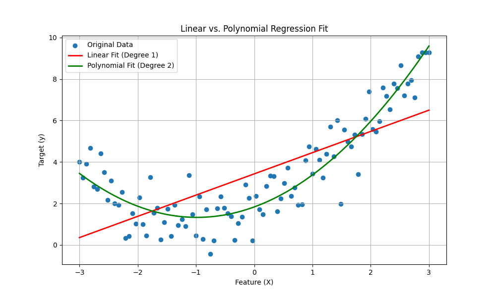
R^2 Score (Linear Fit): 0.5300
R^2 Score (Polynomial Fit): 0.8657
As the visualization and the R² scores show, the simple linear model fails to capture the curve in the data. The polynomial model, by creating an \(x^2\) feature, fits the data significantly better.
Example 2: Creating Interaction Terms
Here, we’ll show how to create interaction terms both manually with pandas and using scikit-learn. We’ll use a hypothetical dataset for predicting ad campaign success.
import pandas as pd
from sklearn.preprocessing import PolynomialFeatures

# 1. Create a sample dataset
data = {
    'ad_spend': [100, 200, 150, 300, 250],
    'time_of_day': [8, 12, 18, 9, 20],  # Hour of the day
    'conversions': [10, 25, 18, 35, 22]
}
df = pd.DataFrame(data)

# 2. Manual creation of interaction term with pandas
df['spend_x_time'] = df['ad_spend'] * df['time_of_day']
print("DataFrame with manually created interaction term:")
print(df)
print("-" * 50)

# 3. Using scikit-learn's PolynomialFeatures for interaction only
# We select the features we want to interact
X = df[['ad_spend', 'time_of_day']]

# interaction_only=True ensures we only get interaction terms (x1*x2), not polynomial terms (x1^2)
interaction_transformer = PolynomialFeatures(degree=2, interaction_only=True, include_bias=False)
X_interact = interaction_transformer.fit_transform(X)

# Convert the result back to a DataFrame for clarity
interact_df = pd.DataFrame(X_interact, columns=interaction_transformer.get_feature_names_out())
print("Features created by scikit-learn (interaction_only=True):")
print(interact_df)
Outputs:
DataFrame with manually created interaction term:
   ad_spend  time_of_day  conversions  spend_x_time
0       100            8           10           800
1       200           12           25          2400
2       150           18           18          2700
3       300            9           35          2700
4       250           20           22          5000
--------------------------------------------------
Features created by scikit-learn (interaction_only=True):
   ad_spend  time_of_day  ad_spend time_of_day
0     100.0          8.0                 800.0
1     200.0         12.0                2400.0
2     150.0         18.0                2700.0
3     300.0          9.0                2700.0
4     250.0         20.0                5000.0
This example illustrates two practical ways to generate interaction terms. The scikit-learn approach is more systematic and scalable, especially when dealing with many features, and integrates seamlessly into modeling pipelines.
Step-by-Step Tutorials
Tutorial: Time-Based Feature Engineering for Sales Data
This tutorial walks through creating a rich set of temporal features from a simple sales dataset. These features are crucial for any time-series forecasting task.
import pandas as pd

# 1. Create a sample sales dataset with a date range
dates = pd.to_datetime(pd.date_range(start='2024-01-01', end='2024-03-31', freq='D'))
np.random.seed(0)
sales = np.random.randint(50, 200, size=len(dates)) + np.arange(len(dates)) * 1.5
sales_df = pd.DataFrame({'sale_date': dates, 'sales': sales})
sales_df = sales_df.set_index('sale_date')

print("Original Sales Data (first 5 rows):")
print(sales_df.head())
print("-" * 50)

# 2. Decompose the timestamp into cyclical features
# We extract features directly from the DatetimeIndex
sales_df['day_of_week'] = sales_df.index.dayofweek  # Monday=0, Sunday=6
sales_df['day_of_year'] = sales_df.index.dayofyear
sales_df['month'] = sales_df.index.month
sales_df['quarter'] = sales_df.index.quarter
sales_df['week_of_year'] = sales_df.index.isocalendar().week.astype(int)
sales_df['is_month_start'] = sales_df.index.is_month_start.astype(int)
sales_df['is_month_end'] = sales_df.index.is_month_end.astype(int)

print("Data with Cyclical Features (first 5 rows):")
print(sales_df.head())
print("-" * 50)

# 3. Create rolling window features
# These features summarize past data over a specific window
sales_df['rolling_mean_7d'] = sales_df['sales'].rolling(window=7).mean()
sales_df['rolling_std_7d'] = sales_df['sales'].rolling(window=7).std()
sales_df['rolling_max_14d'] = sales_df['sales'].rolling(window=14).max()

# 4. Create lag features
# Lag features are the values from previous time steps
sales_df['lag_1d'] = sales_df['sales'].shift(1)
sales_df['lag_7d'] = sales_df['sales'].shift(7)

# The first few rows will have NaNs due to the rolling/lag calculations
# In a real application, these would need to be handled (e.g., filled or dropped)
print("Data with Rolling and Lag Features (showing rows 10-15):")
print(sales_df.iloc[10:16])
Outputs:
Original Sales Data (first 5 rows):
            sales
sale_date
2024-01-01   97.0
2024-01-02  168.5
2024-01-03  120.0
2024-01-04  157.5
2024-01-05   65.0
--------------------------------------------------
Data with Cyclical Features (first 5 rows):
            sales  day_of_week  day_of_year  month  quarter  week_of_year  is_month_start  is_month_end
sale_date
2024-01-01   97.0            0            1      1        1             1               1             0
2024-01-02  168.5            1            2      1        1             1               0             0
2024-01-03  120.0            2            3      1        1             1               0             0
2024-01-04  157.5            3            4      1        1             1               0             0
2024-01-05   65.0            4            5      1        1             1               0             0
--------------------------------------------------
Data with Rolling and Lag Features (showing rows 10-15):
            sales  day_of_week  day_of_year  month  quarter  ...  rolling_mean_7d  rolling_std_7d  rolling_max_14d  lag_1d  lag_7d
sale_date                                                    ...
2024-01-11  205.0            3           11      1        1  ...       124.928571       48.853035              NaN   151.5   157.5
2024-01-12  124.5            4           12      1        1  ...       133.428571       41.276939              NaN   205.0    65.0
2024-01-13  107.0            5           13      1        1  ...       137.500000       36.027767              NaN   124.5    78.5
2024-01-14  156.5            6           14      1        1  ...       146.285714       31.097772            205.0   107.0    95.0
2024-01-15  159.0            0           15      1        1  ...       147.928571       31.474101            205.0   156.5   147.5
2024-01-16  153.5            1           16      1        1  ...       151.000000       30.700163            205.0   159.0   132.0

[6 rows x 13 columns]
This step-by-step process transforms a simple two-column dataset into a rich feature set ready for a sophisticated time-series model. Each new feature provides a different view of the data’s history and structure.
Integration and Deployment Examples
Using Pipeline and ColumnTransformer for Production
In a production environment, it is critical that the exact same feature engineering steps applied during training are applied to new data at inference time. Manually managing these steps is error-prone. Scikit-learn’s Pipeline and ColumnTransformer are the industry-standard tools for creating robust, reproducible preprocessing workflows.
This example shows how to build a pipeline that applies different transformations (scaling and polynomial features) to different columns of a dataset.
import pandas as pd
from sklearn.model_selection import train_test_split
from sklearn.preprocessing import StandardScaler, PolynomialFeatures
from sklearn.compose import ColumnTransformer
from sklearn.linear_model import LogisticRegression
from sklearn.pipeline import Pipeline

# 1. Create a sample dataset for a classification task
data = {
    'age': [25, 45, 35, 50, 23, 65, 33, 42],
    'income': [50000, 120000, 80000, 150000, 45000, 95000, 65000, 110000],
    'product_views': [10, 5, 8, 15, 12, 4, 9, 11],
    'purchased': [0, 1, 1, 1, 0, 0, 0, 1]
}
df = pd.DataFrame(data)
X = df[['age', 'income', 'product_views']]
y = df['purchased']

# 2. Define which columns get which transformations
# We will scale numeric features and create polynomial/interaction terms for others
numeric_features = ['income']
poly_features = ['age', 'product_views']

# 3. Create the preprocessing pipeline using ColumnTransformer
# This applies specific transformers to specific columns
preprocessor = ColumnTransformer(
    transformers=[
        ('num', StandardScaler(), numeric_features),
        ('poly', PolynomialFeatures(degree=2, include_bias=False), poly_features)
    ],
    remainder='passthrough' # Keep other columns (if any)
)

# 4. Create the full pipeline including the model
# The pipeline chains the preprocessor and the classifier
model_pipeline = Pipeline(steps=[
    ('preprocessor', preprocessor),
    ('classifier', LogisticRegression(solver='liblinear', random_state=42))
])

# 5. Train the pipeline on data
X_train, X_test, y_train, y_test = train_test_split(X, y, test_size=0.25, random_state=42)
model_pipeline.fit(X_train, y_train)

# 6. Evaluate the pipeline
accuracy = model_pipeline.score(X_test, y_test)
print(f"Pipeline Accuracy: {accuracy:.4f}")

# 7. Make predictions on new data
# The pipeline handles all transformations automatically
new_data = pd.DataFrame({'age': [38], 'income': [90000], 'product_views': [7]})
prediction = model_pipeline.predict(new_data)
print(f"Prediction for new data: {'Purchased' if prediction[0] == 1 else 'Not Purchased'}")
Outputs:
Pipeline Accuracy: 0.5000
Prediction for new data: Purchased
This pipeline object encapsulates the entire feature engineering and modeling process. It can be saved as a single file (e.g., using joblib) and loaded in a production environment, guaranteeing that the exact same steps are followed, preventing training-serving skew.
Industry Applications and Case Studies
1. Credit Risk Scoring in Financial Services:
- Use Case: Banks and fintech companies build models to predict the likelihood of a borrower defaulting on a loan. The decision to approve or deny a loan, and at what interest rate, is based on this risk assessment.
- Feature Engineering: Raw data includes income, loan amount, age, and employment history. Domain experts create critical features like Debt-to-Income Ratio (\(\frac{\text{Total Monthly Debt}}{\text{Monthly Gross Income}}\)), Loan-to-Value Ratio for mortgages, and Credit History Length. Interaction terms like
age * credit_scoremight capture the idea that a high credit score is more meaningful for a younger applicant. These engineered features provide a much clearer picture of financial health than raw numbers alone. - Business Impact: Improved risk models directly reduce financial losses from defaults and allow for more competitive pricing for low-risk customers, increasing market share.
2. Customer Churn Prediction in Telecommunications:
- Use Case: Mobile and internet providers want to proactively identify customers who are likely to cancel their service. It is far more expensive to acquire a new customer than to retain an existing one.
- Feature Engineering: The raw data consists of call records, data usage logs, billing information, and customer service interactions. Key engineered features include “days since last contract renewal,” “rolling 3-month average of data overage charges,” “number of customer support tickets in the last quarter,” and “ratio of outgoing to incoming calls.” These features capture trends in behavior and dissatisfaction that signal churn risk.
- Business Impact: By identifying at-risk customers, companies can target them with retention offers (e.g., discounts, plan upgrades), significantly reducing churn rates and preserving millions in recurring revenue.
3. Demand Forecasting in Retail and E-commerce:
- Use Case: Retailers need to accurately predict the demand for thousands of products at different locations to optimize inventory, prevent stockouts, and minimize holding costs.
- Feature Engineering: The primary data is historical sales records. This is augmented with information on promotions, holidays, and store locations. The most critical engineered features are temporal. These include “day_of_week,” “is_holiday,” “is_promotional_period,” and various rolling window statistics (e.g., “7-day moving average of sales,” “sales from the same day last year”). Geospatial features like “distance to nearest competitor” can also be added.
- Business Impact: Accurate demand forecasting leads to a more efficient supply chain, higher sales from improved product availability, and lower costs due to reduced overstocking and waste, directly boosting profit margins.
Best Practices and Common Pitfalls
1. Avoid Data Leakage at All Costs:
- Pitfall: A common and severe mistake is to perform feature engineering on the entire dataset before splitting it into training and testing sets. For example, if you calculate the mean of a feature for scaling, using the entire dataset means information from the test set “leaks” into the training process. The model’s performance will be artificially inflated, and it will fail in production.
- Best Practice: Always split your data into training and validation/test sets first. Any feature engineering transformation that learns parameters from the data (like a
StandardScaleror even filling missing values with a mean) must befitonly on the training data and then used totransformboth the training and test data. Using scikit-learnPipelineshelps enforce this practice correctly.
2. Beware the Curse of Dimensionality:
- Pitfall: It can be tempting to generate a massive number of features through automated polynomial and interaction term creation. However, adding too many features (high dimensionality) can make the data sparse, dramatically increase computational requirements, and make the model more likely to overfit by finding spurious correlations in the noise.
- Best Practice: Be selective. Use domain knowledge to guide the creation of interaction terms. Use feature selection techniques (e.g., recursive feature elimination, selection based on feature importance from a tree model) to prune irrelevant or redundant features. Start simple and add complexity iteratively, validating the impact of new features on model performance using cross-validation.
3. Balance Interpretability with Performance:
- Pitfall: Creating highly complex features (e.g., deep polynomial interactions, ratios of ratios) can boost a model’s predictive accuracy by a small margin but make the model a “black box.” In regulated industries like finance and healthcare, being able to explain why a model made a certain prediction is a legal and ethical requirement.
- Best Practice: Understand your project’s requirements. If interpretability is key, favor simpler features whose business meaning is clear (e.g., debt-to-income ratio). Document the logic for every feature created. If pure performance is the only goal, more complex features may be acceptable, but their impact should be carefully measured to justify the loss of transparency.
4. Document Your Feature Creation Process:
- Pitfall: In a complex project, it’s easy to lose track of how dozens or hundreds of features were created. This “feature debt” makes the system difficult to maintain, debug, or hand over to other team members.
- Best Practice: Maintain a feature dictionary or a centralized script with clear comments that serves as the single source of truth for all feature definitions. For each feature, document its name, a clear description of what it represents, the exact formula or code used to generate it, and the rationale for its creation. This documentation is crucial for collaboration, debugging, and model governance.
Hands-on Exercises
1. Basic: Exploring Polynomial Features on a New Dataset
- Objective: Apply polynomial feature transformation and observe its effect on model fit.
- Task:
- Load the “Boston Housing” dataset (available in many libraries, or use a similar regression dataset).
- Select a single feature that appears to have a non-linear relationship with the target variable (e.g., ‘LSTAT’ vs. ‘MEDV’).
- Build and evaluate a simple linear regression model using only this feature.
- Build a second model using a pipeline that includes
PolynomialFeatures(try degrees 2 and 3) andLinearRegression. - Compare the R² scores and plot the regression lines for all three models against the data.
- Expected Outcome: A report or notebook showing that the polynomial models provide a better fit to the data, quantified by a higher R² score and a more visually accurate regression line.
2. Intermediate: Manual Feature Engineering for a Classification Task
- Objective: Use domain intuition to manually create and test features for a classification model.
- Task:
- Use the “Titanic” dataset.
- Create at least three new features based on your hypotheses about survival. Examples:
FamilySize: Sum of ‘SibSp’ and ‘Parch’ plus 1 (for the person themselves).IsAlone: A binary feature based onFamilySize.Title: Extract the title (Mr., Mrs., Miss., etc.) from the ‘Name’ column.
- Preprocess the data (handle missing values, encode categorical features).
- Train a classification model (e.g.,
LogisticRegressionorRandomForestClassifier) on the dataset without your new features. Record its accuracy. - Train the same model on the dataset with your new features.
- Expected Outcome: A comparison of the model’s cross-validated accuracy before and after adding the engineered features, demonstrating an improvement in performance.
3. Advanced: Time-Series Feature Engineering for Forecasting (Team Project)
- Objective: Develop a comprehensive feature set for a real-world time-series forecasting problem.
- Task:
- Find a suitable time-series dataset (e.g., daily retail sales, hourly energy consumption, or stock prices).
- As a team, brainstorm and implement a wide range of temporal features, including:
- Cyclical features (day of week, month, etc.).
- Lag features (value from t-1, t-7, etc.).
- Rolling window features (mean, std, min, max over various windows).
- Any other domain-specific features you can devise (e.g., for a retail dataset, flag the days leading up to a major holiday).
- Split the data chronologically into a training and a test set.
- Train a forecasting model (like a Gradient Boosting Regressor) using your engineered features.
- Evaluate your model’s performance on the test set using metrics like Mean Absolute Error (MAE).
- Expected Outcome: A working forecasting model and a presentation explaining the features created, which ones were most important (using feature importance plots), and the final performance of the model.
Tools and Technologies
The primary toolkit for feature engineering in Python is centered around a few key libraries:
- pandas: The cornerstone for data manipulation in Python. Its
DataFrameobject is the standard for holding and transforming tabular data. It provides a rich API for creating, deleting, and modifying columns, which is the essence of feature engineering. Its time-series functionalities, including functions for resampling, shifting, and rolling windows, are particularly powerful. - NumPy: The fundamental package for scientific computing. It provides efficient array objects and a vast library of mathematical functions that are often used in the backend by pandas and scikit-learn to perform numerical computations required for creating features.
- scikit-learn: The most important machine learning library in Python. While known for its models, its
preprocessingmodule is a treasure trove for feature engineering.PolynomialFeatures: For systematically creating polynomial and interaction terms.StandardScaler,MinMaxScaler: For scaling features, a common subsequent step.Pipeline,ColumnTransformer: Essential tools for building robust and reproducible feature engineering workflows for production.
- Feature-engine: An open-source Python library dedicated exclusively to feature engineering and selection. It provides a wide array of transformers that are compatible with scikit-learn pipelines, covering more advanced techniques for imputation, encoding, and feature creation. It’s a great tool for streamlining and standardizing more complex feature engineering tasks.
- Feature Stores (e.g., Tecton, Feast): In large-scale, production MLOps environments, a feature store is a centralized system that manages the entire lifecycle of features. It handles feature computation, storage, versioning, and serving for both model training (in batches) and real-time inference (with low latency), ensuring consistency and preventing redundant work across different teams and models.
Summary
- Feature Engineering is Critical: It is the process of transforming raw data into informative features that improve machine learning model performance. It is often the most impactful part of the ML pipeline.
- Core Techniques: We covered foundational methods like Polynomial Features to capture non-linearities and Interaction Terms to model feature synergies.
- Domain-Specific Knowledge is Key: The most powerful features often come from understanding the problem domain, especially in creating Temporal Features from timestamps (e.g., date components, rolling windows, and time lags).
- Implementation is Systematic: Libraries like pandas and scikit-learn provide the tools to implement these techniques efficiently and reliably.
- Production Requires Pipelines: For deployment, feature engineering logic must be encapsulated in reproducible workflows using tools like scikit-learn’s
PipelineandColumnTransformerto prevent training-serving skew. - Beware of Pitfalls: Key challenges include avoiding data leakage, managing the curse of dimensionality, and balancing model performance with interpretability.
Further Reading and Resources
- Scikit-learn Documentation: The official documentation for the
sklearn.preprocessingandsklearn.composemodules is the definitive resource for the tools discussed. https://scikit-learn.org/stable/modules/preprocessing.html - “Feature Engineering for Machine Learning: Principles and Techniques for Data Scientists” by Alice Zheng & Amanda Casari: A comprehensive book that provides a principled guide to the entire feature engineering process.
- “Python for Data Analysis, 3rd Edition” by Wes McKinney: The authoritative guide to the pandas library, written by its creator. Essential for mastering the data manipulation skills needed for feature engineering.
- Feature-engine Documentation: Explore the documentation for this specialized library to discover a wider range of pre-built feature engineering transformers. https://feature-engine.readthedocs.io/
- Feast (Open Source Feature Store): The official website and documentation for Feast, a leading open-source feature store, to understand how feature engineering is managed at scale in production MLOps. https://feast.dev/
Glossary of Terms
- Feature Engineering: The process of using domain knowledge to select, transform, and create new variables (features) from raw data to improve machine learning model performance.
- Polynomial Features: New features created by raising existing features to an exponent (e.g., \(x^2, x^3\)). They allow linear models to capture non-linear relationships.
- Interaction Term: A feature created by multiplying two or more existing features. It allows a model to capture the synergistic or antagonistic effects between variables.
- Data Leakage: The introduction of information from outside the training dataset into the model building process, often leading to overly optimistic performance estimates and poor real-world performance.
- Curse of Dimensionality: A term describing the various problems that arise when working with high-dimensional data, such as data sparsity and increased computational complexity, which can degrade model performance.
- Rolling Window (or Moving Average): A technique used in time-series analysis where calculations (e.g., mean, sum, std) are performed on a sliding window of a fixed size over the data to create features that summarize recent trends.
- Lag Feature: A feature in a time-series dataset that contains data from a prior time step (e.g., the sales value from the previous day).
- Pipeline (in scikit-learn): An object that sequentially applies a list of transformers and a final estimator. It is used to chain multiple processing steps together into a single, reproducible workflow.
- ColumnTransformer (in scikit-learn): A tool for applying different transformers to different columns of an array or DataFrame, often used within a Pipeline.
- Feature Store: A centralized data management system for machine learning features, used to store, retrieve, and manage features for both training and serving.
