
Chapter 20: Pandas for Data Manipulation: DataFrames and Series
Chapter Objectives
Upon completing this chapter, you will be able to:
- Understand the fundamental architecture of Pandas, including the Series and DataFrame objects, and their relationship to the underlying NumPy library.
- Implement a wide range of data selection, filtering, and indexing techniques using labels (
.loc), integer positions (.iloc), and boolean masking to precisely access and manipulate data subsets. - Analyze and clean complex datasets by identifying and handling missing values, removing duplicate records, and transforming data types to prepare them for machine learning pipelines.
- Design sophisticated data transformation workflows by applying custom functions, performing vectorized operations, and leveraging the split-apply-combine strategy with
.groupby()for powerful data aggregation. - Optimize data manipulation code for performance by avoiding inefficient loops in favor of vectorized operations and understanding memory management within Pandas.
- Deploy data merging and joining strategies to integrate data from multiple sources into a unified, analysis-ready dataset using
merge,join, andconcatoperations.
Introduction
In the ecosystem of modern AI and machine learning engineering, data is the foundational element—the raw material from which insights are forged and predictive models are built. However, data in its initial state is rarely pristine or structured for immediate use. It is often messy, incomplete, and spread across multiple sources. The process of transforming this raw data into a clean, coherent, and feature-rich format is known as data wrangling or data manipulation, and it is arguably the most critical and time-consuming phase of any AI project. This is where the Pandas library emerges as an indispensable tool for any Python-based data scientist or AI engineer.
Pandas provides high-performance, easy-to-use data structures and data analysis tools that have become the de facto standard for data manipulation in Python. Its core data structures, the Series and the DataFrame, allow for the intuitive handling of tabular data, time series, and other forms of observational datasets. This chapter will serve as a comprehensive guide to mastering Pandas, moving from fundamental concepts to advanced data transformation techniques. We will explore how to load, clean, reshape, merge, and aggregate data with efficiency and precision. By the end of this chapter, you will not only understand the syntax of Pandas but also the underlying logic that makes it a powerhouse for preparing data for sophisticated machine learning algorithms. This foundational skill is paramount, as the quality of your data preparation directly dictates the performance and reliability of the AI systems you build.
Technical Background
The Core Data Structures: Series and DataFrame
At the heart of the Pandas library are two fundamental data structures: the Series and the DataFrame. Understanding their design and interplay is the first step toward mastering data manipulation in Python. These structures were not created in a vacuum; they are built upon the high-performance NumPy array object, which provides the foundation for their speed and memory efficiency. However, Pandas introduces a crucial layer of abstraction on top of NumPy: expressive, flexible labels for rows and columns, which transforms the way we interact with data.
Pandas Series vs. NumPy 1D Array
| Feature | Pandas Series | NumPy 1D Array |
|---|---|---|
| Index | Explicitly defined, flexible index (e.g., strings, dates). Not limited to integers. | Implicitly defined integer index (0, 1, 2, …). |
| Data Types | Can hold heterogeneous data types (though often homogeneous for performance). | Homogeneous data type; all elements must be of the same type (e.g., all int64). |
| Missing Data | Built-in support for missing data, represented as NaN. |
Requires special handling for missing data (e.g., using masked arrays). |
| Data Alignment | Operations automatically align data based on index labels. | Operations are based on element position (index). |
| Metadata | Can have a name attribute for the Series itself and its index. | No built-in support for metadata like names. |
| Use Case | Ideal for labeled, time-series, or tabular column data where index matters. | Best for raw numerical computation and linear algebra. |
The Pandas Series: A Labeled One-Dimensional Array
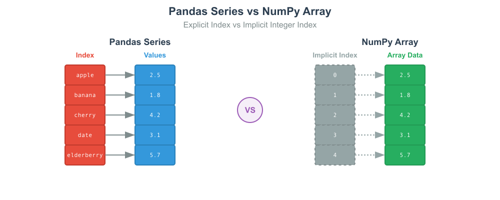
A Series is the simplest Pandas data structure, best conceptualized as a one-dimensional array-like object capable of holding any data type—integers, strings, floating-point numbers, Python objects, and more. What distinguishes a Series from a one-dimensional NumPy array is its index. The index is an associated array of labels that provides a powerful way to reference and access data. While a NumPy array has an implicitly defined integer index, a Pandas Series can have a custom-defined index, which can consist of numbers, strings, or even dates. This explicit indexing allows for more intuitive data alignment and retrieval, making code more readable and less prone to errors.
For example, a Series could represent the population of several cities, where the data points are the population figures and the index labels are the city names. This direct mapping between labels and data is a cornerstone of Pandas’ design philosophy. Mathematically, a Series can be thought of as a mapping of index labels to data values, similar to a Python dictionary but with the performance benefits of contiguous memory allocation inherited from NumPy. Operations on a Series are typically vectorized, meaning that functions are applied to the entire array of data at once without the need for explicit Python loops. This vectorization is a key source of Pandas’ computational efficiency.
The DataFrame: A Two-Dimensional Labeled Structure
The DataFrame is the most commonly used object in Pandas and represents the primary workhorse for data analysis. A DataFrame is a two-dimensional, size-mutable, and potentially heterogeneous tabular data structure with labeled axes (rows and columns). You can think of it as a spreadsheet, an SQL table, or a dictionary of Series objects where each Series shares the same index. A DataFrame has both a row index and a column index, making data access incredibly flexible.
graph TD;
    subgraph NumPy Foundation
        direction LR
        NP_Array1D[("NumPy 1D Array<br><i>(Contiguous Memory)</i>")]
        NP_Array2D[("NumPy 2D Array<br><i>(Contiguous Memory)</i>")]
    end

    subgraph Pandas Objects
        direction TB
        Series[<b>Pandas Series</b><br><i>1D Labeled Array</i>]
        DataFrame[<b>Pandas DataFrame</b><br><i>2D Labeled Table</i>]
    end

    NP_Array1D -->|Built Upon| Series;
    Series -->|Is a Column in| DataFrame;

    subgraph Series Components
        direction LR
        S_Index["Index<br>('city_a', 'city_b', ...)"]
        S_Data["Data<br>(1.2M, 2.5M, ...)"]
    end

    subgraph DataFrame Components
        direction LR
        DF_RowIndex["Row Index<br>('2023-01', '2023-02', ...)"]
        DF_Cols["Columns (Series Objects)"]
    end

    Series -- Composed of --- S_Index;
    Series -- Composed of --- S_Data;
    DataFrame -- Composed of --- DF_RowIndex;
    DataFrame -- Composed of --- DF_Cols;

    style NP_Array1D fill:#ebf5ee,stroke:#283044,stroke-width:2px,color:#283044
    style NP_Array2D fill:#ebf5ee,stroke:#283044,stroke-width:2px,color:#283044
    style Series fill:#283044,stroke:#283044,stroke-width:2px,color:#ebf5ee
    style DataFrame fill:#283044,stroke:#283044,stroke-width:2px,color:#ebf5ee
    style S_Index fill:#9b59b6,stroke:#9b59b6,stroke-width:1px,color:#ebf5ee
    style S_Data fill:#9b59b6,stroke:#9b59b6,stroke-width:1px,color:#ebf5ee
    style DF_RowIndex fill:#9b59b6,stroke:#9b59b6,stroke-width:1px,color:#ebf5ee
    style DF_Cols fill:#78a1bb,stroke:#78a1bb,stroke-width:1px,color:#283044
Each column in a DataFrame is a Series, and all columns share the same row index. This structure allows for powerful data alignment capabilities. When performing operations between DataFrames or between a DataFrame and a Series, Pandas automatically aligns the data based on the index and column labels. This feature prevents many common errors that arise from misaligned data in other tools and is particularly useful when working with incomplete or messy datasets. For instance, if you add two DataFrames, Pandas will match the rows and columns by their labels and perform the addition only on the matching cells, propagating NaN (Not a Number) for any non-overlapping labels. This automatic alignment is a powerful feature for ensuring data integrity during complex transformations. The ability to handle heterogeneous data types—having columns of integers, floats, strings, and booleans within the same table—makes the DataFrame an exceptionally versatile tool for real-world data.

Data Indexing and Selection
Effective data analysis requires the ability to precisely select, slice, and filter subsets of data. Pandas provides a rich and powerful set of tools for this purpose, primarily through its indexing operators. While the syntax may initially seem complex, mastering these methods is essential for efficient data manipulation. The primary access methods are label-based indexing with .loc, integer position-based indexing with .iloc, and boolean masking.
Label-Based Selection with .loc
The .loc indexer is the primary method for label-based data selection. It allows you to select data based on the explicit index and column labels you have defined. The syntax .loc[row_labels, column_labels] is both intuitive and powerful. You can pass single labels, lists of labels, or slice objects with labels. For example, df.loc['Row_1', 'Column_A'] would select the single value at the intersection of that row and column. A slice like df.loc['Row_1':'Row_5', ['Column_A', 'Column_C']] would select rows 1 through 5 (inclusive of both endpoints) and specifically columns A and C.
The key advantage of .loc is its explicitness. Your code refers to data by its semantic labels, making it more readable and robust to changes in the data’s ordering. If the rows of your DataFrame are shuffled, code using .loc will still select the correct data because it relies on the immutable labels, not the transient integer position. This is crucial for writing reproducible and maintainable analysis scripts.
Warning: When using slices with
.loc, the start and end bounds are both included in the result. This differs from standard Python slicing of lists or integer-based slicing with.iloc, where the end bound is exclusive.
Positional Selection with .iloc
In contrast to .loc, the .iloc indexer is used for integer position-based indexing. It works just like standard Python list slicing, where you refer to rows and columns by their integer position (starting from 0). The syntax is .iloc[row_positions, column_positions]. For example, df.iloc[0, 0] selects the data in the very first row and first column, regardless of what their labels are. A slice like df.iloc[0:5, [0, 2]] would select the first five rows (from position 0 up to, but not including, 5) and the first and third columns.
.iloc is useful when you need to access data by its position or when your DataFrame does not have meaningful labels. However, it can be brittle. If the order of columns or rows changes, your .iloc-based code may select the wrong data without raising an error. Therefore, it is often recommended to prefer .loc for clarity and safety unless you have a specific reason to rely on integer positions.
Comparison of Pandas Indexers: .loc vs. .iloc
| Aspect | .loc (Label-Based) |
.iloc (Integer-Based) |
|---|---|---|
| Primary Use | Selection by explicit index labels and column names. | Selection by integer position (from 0 to length-1). |
| Input Types | Labels (strings, numbers if the index is numeric), lists of labels, boolean arrays, slices with labels. | Integers, lists of integers, boolean arrays, slices with integers. |
| Slicing Behavior | Endpoint is inclusive. df.loc['a':'c'] includes ‘c’. |
Endpoint is exclusive. df.iloc[0:3] includes positions 0, 1, 2. |
| Robustness | More robust and readable. Code is not affected by changes in row/column order. | Can be brittle. Code may break or select wrong data if row/column order changes. |
| Example | df.loc['row_label', 'col_name'] |
df.iloc[0, 1] |
| When to Use | When your index has meaningful labels. This is the preferred method for clarity. | When you need to select by position, or when the index is not meaningful or is duplicated. |
Boolean Indexing: The Power of Filtering
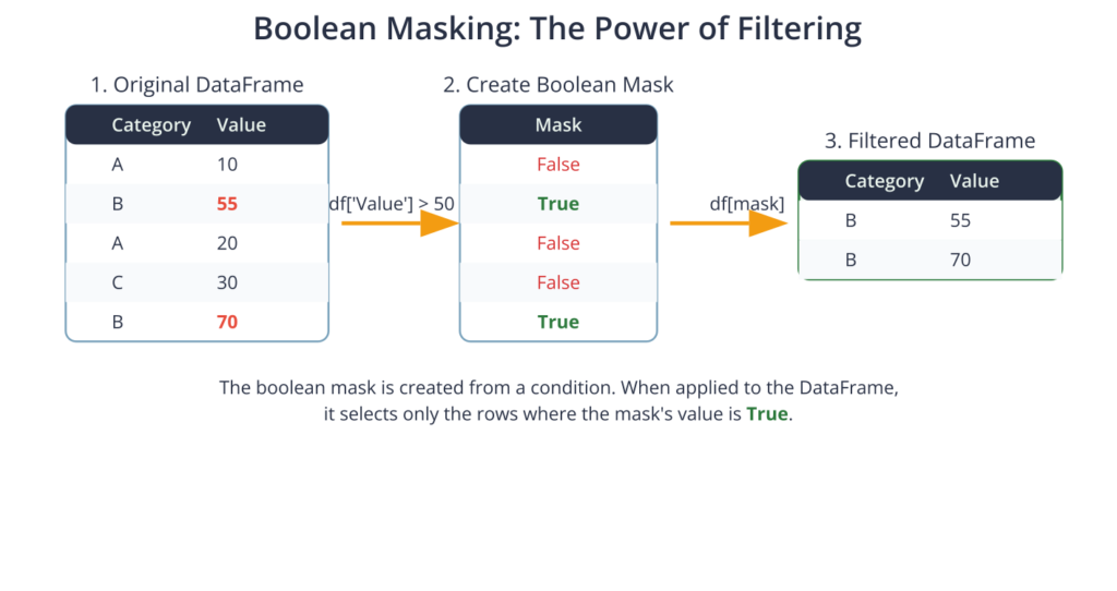
Boolean indexing, or boolean masking, is one of the most powerful and frequently used selection methods in Pandas. It allows you to filter your data based on its actual values rather than just its labels or positions. The process involves creating a Series of boolean values (True/False) that is the same length as the DataFrame’s index. This boolean Series, often called a mask, is then passed to the indexing operator (usually [] or .loc) to select only the rows where the mask’s value is True.
For example, to select all rows from a DataFrame df where the value in ‘Column_A’ is greater than 50, you would write df[df['Column_A'] > 50]. The expression df['Column_A'] > 50 first evaluates to a boolean Series (e.g., [False, True, True, False, ...]). When this mask is passed to df[], it returns a new DataFrame containing only the rows that correspond to a True value. You can combine multiple conditions using logical operators: & for AND, | for OR, and ~ for NOT. For complex conditions, it is essential to wrap each individual condition in parentheses due to Python’s operator precedence rules (e.g., df[(df['col_A'] > 50) & (df['col_B'] == 'Category_X')]). This technique is fundamental for data cleaning, outlier detection, and preparing specific data subsets for analysis.
Grouping and Aggregation: The Split-Apply-Combine Strategy
A cornerstone of data analysis is the ability to summarize and compute statistics on groups of data. Pandas provides a flexible and powerful mechanism for this through its .groupby() method, which implements the highly influential split-apply-combine strategy. This three-step process allows you to perform complex, group-specific calculations that would be cumbersome to implement manually.
The process begins with the split step. When you call df.groupby('column_name'), Pandas inspects the values in the specified column(s) and partitions the DataFrame into smaller DataFrames, one for each unique value or combination of values in the grouping key(s). These sub-DataFrames are not created in memory immediately; instead, groupby creates a DataFrameGroupBy object, which is a lightweight object that holds all the information needed to process the groups.
Next is the apply step. In this stage, a function is applied to each of the individual groups. This function can be an aggregation function that summarizes the data in the group (like .sum(), .mean(), .count()), a transformation function that performs some group-specific computation and returns a result of the same shape (like .transform()), or a filtration function that discards entire groups based on some computation (.filter()). The power of groupby lies in its ability to apply nearly any function you can conceive to each data subset independently.
Finally, the combine step reassembles the results from the apply step into a single, coherent data structure. If an aggregation function was used, the result is typically a new DataFrame where the index is composed of the unique group keys. For example, df.groupby('Category').agg({'Value': 'sum'}) would return a DataFrame with ‘Category’ as the index and the sum of ‘Value’ for each category as the data. This split-apply-combine pattern is incredibly versatile and forms the basis for many complex data analysis tasks, from calculating summary statistics for different experimental conditions to creating features for machine learning models based on categorical variables.
graph TD
    A[<b>Start: Full DataFrame</b>] --> B{Split by Category};

    subgraph " "
        direction LR
        B --> G1[Group A DataFrame];
        B --> G2[Group B DataFrame];
        B --> G3[Group C DataFrame];
    end

    subgraph Apply Function
        G1 --> F1["Apply: .mean()"];
        G2 --> F2["Apply: .mean()"];
        G3 --> F3["Apply: .mean()"];
    end

    subgraph " "
        direction LR
        F1 --> R1[Result A];
        F2 --> R2[Result B];
        F3 --> R3[Result C];
    end

    R1 --> Z{Combine};
    R2 --> Z;
    R3 --> Z;

    Z --> E[<b>End: Aggregated DataFrame</b>];

    classDef start fill:#283044,stroke:#283044,stroke-width:2px,color:#ebf5ee;
    classDef endo fill:#2d7a3d,stroke:#2d7a3d,stroke-width:2px,color:#ebf5ee;
    classDef decision fill:#f39c12,stroke:#f39c12,stroke-width:1px,color:#283044;
    classDef process fill:#78a1bb,stroke:#78a1bb,stroke-width:1px,color:#283044;
    classDef data fill:#9b59b6,stroke:#9b59b6,stroke-width:1px,color:#ebf5ee;
    classDef model fill:#e74c3c,stroke:#e74c3c,stroke-width:1px,color:#ebf5ee;

    class A start;
    class B decision;
    class G1,G2,G3 data;
    class F1,F2,F3 process;
    class R1,R2,R3 model;
    class Z decision;
    class E endo;
Merging, Joining, and Concatenating DataFrames
In real-world AI projects, data rarely comes from a single, clean source. It is often spread across multiple files or database tables that need to be combined. Pandas provides a comprehensive toolkit for this purpose, offering several functions to merge and concatenate DataFrames with logic similar to relational database operations like SQL joins. The primary functions for combining DataFrames are pd.concat(), pd.merge(), and the .join() method.
Concatenation with pd.concat() is the simplest way to combine DataFrames. It works by stacking DataFrames either vertically (axis=0, the default) or horizontally (axis=1). When concatenating vertically, Pandas appends rows from one DataFrame to another. It’s crucial that the columns align; if the DataFrames have different columns, Pandas will fill the missing values with NaN by default. This is useful for combining datasets that have the same structure, such as monthly sales reports.
Merging with pd.merge() is used for more complex, database-style joins. It combines DataFrames based on the values in one or more common columns, known as join keys. The merge function is highly flexible and supports all standard join types:
- Inner Join (default): Returns only the rows where the key exists in both DataFrames. This is the intersection of the keys.
- Outer Join: Returns all rows from both DataFrames. If a key from one DataFrame doesn’t exist in the other, the corresponding columns from the other DataFrame will be filled with
NaN. This is the union of the keys. - Left Join: Returns all rows from the left DataFrame and only the matching rows from the right DataFrame. If a key from the left DataFrame has no match in the right, the right-side columns will be
NaN. - Right Join: Returns all rows from the right DataFrame and only the matching rows from the left.
The .join() method is a convenient alternative to merge that joins DataFrames based on their indices by default, though it can also join on columns. It is essentially a specialized version of merge optimized for index-based joins. Choosing the right method depends on the specific task: use concat for simple stacking, and merge or join for combining datasets based on common keys or indices.
Pandas Data Combination Methods
| Method | Primary Use Case | How it Works | Key Parameters |
|---|---|---|---|
pd.concat() |
Stacking DataFrames vertically (appending rows) or horizontally (adding columns). | Aligns based on index (for horizontal) or columns (for vertical). | axis, join, ignore_index |
pd.merge() |
SQL-style joins. Combining DataFrames based on common column values. | Finds matching values in one or more key columns to align rows. | on, how, left_on, right_on |
df.join() |
A convenient method for index-based merges (or joining on a column to an index). | Aligns the calling DataFrame’s index with the other DataFrame’s index or key column(s). | on, how |
Practical Examples and Implementation
Mathematical Concept Implementation
Many Pandas operations are practical implementations of underlying mathematical and statistical concepts. For instance, the .mean() method directly computes the arithmetic mean, \(\bar{x} = \frac{1}{n}\sum_{i=1}^{n}x_i\), across a Series or DataFrame axis. Let’s demonstrate this and other concepts using Python.
We’ll start by creating a DataFrame and calculating some basic descriptive statistics, which are fundamental in the exploratory data analysis (EDA) phase of any ML project.
import pandas as pd
import numpy as np

# Create a sample DataFrame
data = {
    'Category': ['A', 'B', 'A', 'B', 'A', 'C'],
    'Value1': [10, 15, 12, 18, 11, 25],
    'Value2': [100, 110, 105, 115, 102, 120]
}
df = pd.DataFrame(data)

print("Original DataFrame:")
print(df)

# --- Mathematical/Statistical Operations ---

# Calculating the mean (arithmetic average)
mean_value1 = df['Value1'].mean()
print(f"\nMean of Value1: {mean_value1:.2f}")

# Calculating standard deviation
# Formula: sqrt( (1/N) * sum( (x_i - mu)^2 ) )
std_dev_value1 = df['Value1'].std()
print(f"Standard Deviation of Value1: {std_dev_value1:.2f}")

# Calculating correlation between two columns
# Correlation coefficient 'r' measures linear relationship
correlation = df['Value1'].corr(df['Value2'])
print(f"Correlation between Value1 and Value2: {correlation:.2f}")

# The .describe() method provides a summary of these statistics
print("\nDescriptive Statistics using .describe():")
print(df.describe())
Outputs:
Original DataFrame:
  Category  Value1  Value2
0        A      10     100
1        B      15     110
2        A      12     105
3        B      18     115
4        A      11     102
5        C      25     120

Mean of Value1: 15.17
Standard Deviation of Value1: 5.64
Correlation between Value1 and Value2: 0.97

Descriptive Statistics using .describe():
          Value1      Value2
count   6.000000    6.000000
mean   15.166667  108.666667
std     5.636193    7.788881
min    10.000000  100.000000
25%    11.250000  102.750000
50%    13.500000  107.500000
75%    17.250000  113.750000
max    25.000000  120.000000
This code shows how single lines of Pandas code execute statistical computations that are foundational to understanding data distributions and relationships before feeding them into a model. The .corr() method, for example, computes the Pearson correlation coefficient, a measure of linear association between two variables, which is crucial for feature selection.
AI/ML Application Examples
Let’s walk through a more realistic example: preparing data for a machine learning model. A common task is feature engineering, where we create new variables from existing ones. We’ll also perform one-hot encoding on a categorical variable, a necessary step for many algorithms that cannot handle non-numeric input.
We’ll use a sample dataset representing customer information to predict churn.
import pandas as pd

# Sample customer dataset
data = {
    'CustomerID': [101, 102, 103, 104, 105],
    'Age': [25, 45, 31, 22, 54],
    'Plan': ['Basic', 'Premium', 'Basic', 'Gold', 'Premium'],
    'MonthlySpend': [50, 120, 55, 90, 130],
    'Churn': [0, 1, 0, 0, 1] # 1 for churn, 0 for no churn
}
customer_df = pd.DataFrame(data)

print("Original Customer DataFrame:")
print(customer_df)

# --- Feature Engineering ---
# Create a new feature: 'AgeGroup'
bins = [18, 30, 50, 100]
labels = ['Young Adult', 'Adult', 'Senior']
customer_df['AgeGroup'] = pd.cut(customer_df['Age'], bins=bins, labels=labels, right=False)

print("\nDataFrame with new 'AgeGroup' feature:")
print(customer_df)

# --- Data Cleaning: Handling Missing Values (Hypothetical) ---
# Let's add a missing value to demonstrate cleaning
customer_df.loc[2, 'MonthlySpend'] = np.nan
print("\nDataFrame with missing value:")
print(customer_df)

# Impute the missing value with the mean of the column
mean_spend = customer_df['MonthlySpend'].mean()
customer_df['MonthlySpend'].fillna(mean_spend, inplace=True)
print("\nDataFrame after imputing missing value:")
print(customer_df)


# --- One-Hot Encoding for Categorical Variable 'Plan' ---
# This converts categorical variables into a numerical format
plan_dummies = pd.get_dummies(customer_df['Plan'], prefix='Plan')

# Join the new dummy variables back to the original DataFrame
customer_df_encoded = pd.concat([customer_df, plan_dummies], axis=1)

# Drop the original 'Plan' column and other non-numeric identifiers
customer_df_encoded.drop(['Plan', 'CustomerID', 'AgeGroup'], axis=1, inplace=True)

print("\nFinal DataFrame ready for Machine Learning:")
print(customer_df_encoded)
Outputs:
DataFrame after imputing missing value:
   CustomerID  Age     Plan  MonthlySpend  Churn     AgeGroup
0         101   25    Basic          50.0      0  Young Adult
1         102   45  Premium         120.0      1        Adult
2         103   31    Basic          97.5      0        Adult
3         104   22     Gold          90.0      0  Young Adult
4         105   54  Premium         130.0      1       Senior

Final DataFrame ready for Machine Learning:
   Age  MonthlySpend  Churn  Plan_Basic  Plan_Gold  Plan_Premium
0   25          50.0      0        True      False         False
1   45         120.0      1       False      False          True
2   31          97.5      0        True      False         False
3   22          90.0      0       False       True         False
4   54         130.0      1       False      False          True
In this example, we performed several key data preparation steps. We created a new categorical feature AgeGroup from the continuous Age variable, a process known as binning. We then demonstrated how to handle missing data by imputing the mean value. Finally, we used pd.get_dummies to perform one-hot encoding, transforming the Plan column into three binary columns. The final customer_df_encoded DataFrame contains only numeric data and is in the correct format to be used as input for a scikit-learn model.
Visualization and Interactive Examples
Visualizing data is crucial for gaining intuition. Pandas integrates seamlessly with visualization libraries like Matplotlib and Seaborn. Let’s visualize the distribution of our Value1 column and explore the relationship between Value1 and Value2.
import pandas as pd
import numpy as np
import matplotlib.pyplot as plt
import seaborn as sns

# Use the first DataFrame from the previous section
data = {
    'Category': ['A', 'B', 'A', 'B', 'A', 'C'],
    'Value1': [10, 15, 12, 18, 11, 25],
    'Value2': [100, 110, 105, 115, 102, 120]
}
df = pd.DataFrame(data)

# Set a nice style for the plots
sns.set_style("whitegrid")

# --- Visualization 1: Distribution of a single variable ---
plt.figure(figsize=(10, 5))
sns.histplot(df['Value1'], kde=True, bins=5)
plt.title('Distribution of Value1')
plt.xlabel('Value1')
plt.ylabel('Frequency')
plt.show()

# --- Visualization 2: Relationship between two variables ---
plt.figure(figsize=(10, 5))
sns.scatterplot(x='Value1', y='Value2', data=df)
plt.title('Relationship between Value1 and Value2')
plt.xlabel('Value1')
plt.ylabel('Value2')
plt.show()

# --- Visualization 3: Grouped analysis ---
# Boxplot to compare distributions of Value1 across categories
plt.figure(figsize=(10, 5))
sns.boxplot(x='Category', y='Value1', data=df)
plt.title('Distribution of Value1 by Category')
plt.xlabel('Category')
plt.ylabel('Value1')
plt.show()
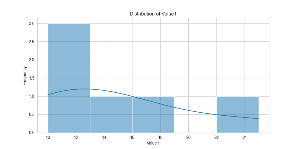
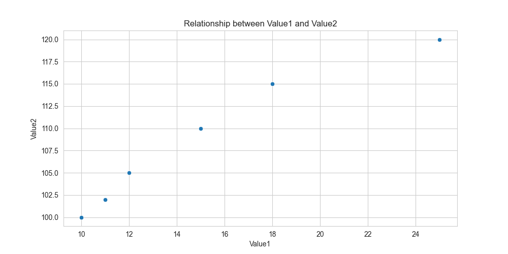
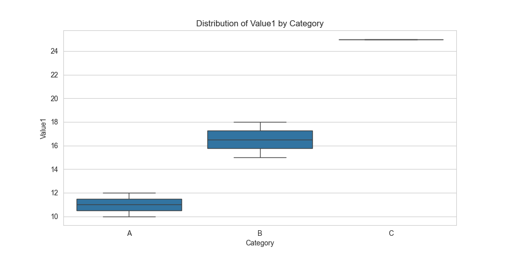
These visualizations allow us to quickly grasp key characteristics of the data. The histogram shows the shape of the Value1 distribution. The scatter plot suggests a positive linear relationship between Value1 and Value2, which aligns with our earlier correlation calculation. The boxplot provides a powerful way to compare the statistical summary (median, quartiles, outliers) of Value1 for each category, revealing insights that might be missed by looking at raw numbers alone.
Computational Exercises
To solidify your understanding, let’s work through a hands-on exercise. Given the following DataFrame of student grades, perform the tasks below.
import pandas as pd

grades_data = {
    'StudentID': range(1, 11),
    'Major': ['CS', 'EE', 'CS', 'ME', 'EE', 'CS', 'ME', 'CS', 'EE', 'ME'],
    'Midterm': [85, 90, 78, 88, 92, 81, 76, 89, 94, 84],
    'Final': [92, 88, 81, 90, 95, 86, 79, 93, 97, 85]
}
grades_df = pd.DataFrame(grades_data)Tasks:
- Calculate Overall Score: Create a new column named
Overallwhich is the average of theMidtermandFinalgrades. - Filter Top Performers: Create a new DataFrame called
top_studentsthat includes only the students whoseOverallscore is 90 or higher. - Analyze Performance by Major: Using
groupby(), calculate the averageMidterm,Final, andOverallscore for eachMajor.
Solution:
# Task 1: Calculate Overall Score
grades_df['Overall'] = (grades_df['Midterm'] + grades_df['Final']) / 2
print("DataFrame with Overall Score:")
print(grades_df)

# Task 2: Filter Top Performers
top_students = grades_df[grades_df['Overall'] >= 90]
print("\nTop Performing Students (Overall >= 90):")
print(top_students)

# Task 3: Analyze Performance by Major
major_performance = grades_df.groupby('Major')[['Midterm', 'Final', 'Overall']].mean()
print("\nAverage Performance by Major:")
print(major_performance.round(2))
This exercise reinforces several core skills: creating new columns from existing data, using boolean indexing for filtering, and performing grouped aggregations to derive summary insights. These are routine tasks in any data analysis workflow.
Industry Applications and Case Studies
Pandas is not just an academic tool; it is the bedrock of data analysis in countless industries, driving business decisions and powering AI systems. Its versatility makes it applicable to nearly any domain where data is collected.
- Finance and Algorithmic Trading: In the financial sector, Pandas is used extensively for time-series analysis. Quantitative analysts use it to process vast amounts of historical stock price data, backtest trading strategies, and calculate financial metrics like moving averages and volatility. A common use case involves loading minute-by-minute tick data into a DataFrame, resampling it to different time frequencies (e.g., daily, hourly), and then merging it with economic indicator data to build predictive models for market movements. The challenge here is performance, as financial datasets can be enormous, requiring optimized, vectorized code.
- E-commerce and Customer Analytics: Online retailers leverage Pandas to understand customer behavior and personalize experiences. They analyze clickstream data, purchase history, and user demographics to segment customers. For example, an e-commerce company might use
groupby()to aggregate purchase data by customer ID to calculate metrics like lifetime value (LTV) or purchase frequency. They could then merge this with product information to build recommendation engines. The business impact is direct: improved customer targeting, increased sales, and reduced churn. - Biotechnology and Genomics: The field of bioinformatics deals with massive datasets from DNA sequencing and other biological experiments. Pandas is used to parse, clean, and analyze this data. A researcher might load a gene expression dataset into a DataFrame, where rows represent genes and columns represent different samples or conditions. They would then filter for significantly expressed genes, merge the data with gene annotation databases, and perform statistical analyses to identify genes associated with a particular disease. Here, the ability of Pandas to handle diverse data types and integrate data from various sources is critical.
- Logistics and Supply Chain Optimization: Companies like FedEx or Amazon analyze operational data to optimize their supply chains. They use Pandas to process data from sensors, vehicle GPS, and warehouse management systems. A typical application would be to analyze delivery route data to identify inefficiencies. By merging route data with traffic patterns and delivery time windows, they can model and optimize future routes, reducing fuel costs and improving delivery times.
Best Practices and Common Pitfalls
While Pandas is powerful, using it effectively and efficiently requires adherence to certain best practices and an awareness of common pitfalls. Writing clean, performant Pandas code is a hallmark of a skilled AI engineer.
- Embrace Vectorization, Avoid Loops: The single most important performance practice in Pandas is to use its built-in vectorized operations instead of iterating over DataFrame rows with Python loops (
for row in df.itertuples():). Operations applied to an entire Series or DataFrame at once are executed in highly optimized C code at the backend, making them orders of magnitude faster than a manual Python loop. For conditional logic, use functions likenp.whereor boolean masking instead ofif/elsestatements inside a loop. - Beware of
SettingWithCopyWarning: This is one of the most common sources of confusion for new Pandas users. This warning appears when you try to assign a value to a slice of a DataFrame that might be a copy rather than a view. For example,df[df['A'] > 0]['B'] = 99is ambiguous. Pandas cannot guarantee whether the first selectiondf[df['A'] > 0]returns a view or a copy of the original data. The assignment might therefore fail silently. The robust solution is to use.locfor assignment:df.loc[df['A'] > 0, 'B'] = 99. This syntax explicitly tells Pandas to modify the original DataFramedfat the specified locations. - Manage Memory Usage: DataFrames can consume significant memory, especially with large datasets. Use appropriate data types. If a column of integers only contains small numbers, you can downcast it from the default
int64toint32orint16using.astype(). For categorical columns with a small number of unique values, converting the type tocategory(df['col'].astype('category')) can lead to massive memory savings and performance improvements, as Pandas will store the data as integer codes rather than repeating strings. - Use Method Chaining for Readability: For a sequence of data manipulation steps, chaining methods together can produce highly readable and efficient code. Instead of creating intermediate DataFrames at each step, you can write a single, fluid expression.
# Instead of this: # df1 = df[df['col_A'] > 50] # df2 = df1.groupby('Category') # result = df2['Value'].mean() # Use this: result = (df[df['col_A'] > 50] .groupby('Category')['Value'] .mean() .reset_index())Wrapping the entire chain in parentheses allows you to format it across multiple lines for clarity. - Understand
inplaceOperations with Caution: Many Pandas methods have aninplace=Trueparameter, which modifies the DataFrame directly instead of returning a new one. While this can seem more memory-efficient, it is often discouraged in modern Pandas code. It can lead to unexpected side effects, especially within complex function calls, and breaks the clean, linear flow of method chaining. The recommended practice is to favor the defaultinplace=Falseand assign the result to a new variable or overwrite the old one:df = df.dropna().
Hands-on Exercises
- Basic Data Exploration:
- Objective: Load a dataset and perform initial exploratory analysis.
- Task: Load the classic Iris dataset, which is available directly from the Seaborn library (sns.load_dataset(‘iris’)).a. Display the first 10 rows of the DataFrame.b. Use .info() to check the data types and look for missing values.c. Use .describe() to get summary statistics for the numerical columns.d. Find the number of unique species in the species column using .nunique().
- Success Criteria: You have successfully loaded the data and can articulate its basic properties, such as the number of samples, features, and data types.
- Intermediate Filtering and Transformation:
- Objective: Practice advanced filtering and data transformation.
- Task: Using the Iris dataset from Exercise 1:a. Create a new DataFrame containing only the flowers of the virginica species.b. From this new DataFrame, filter it further to include only the flowers with a sepal_width greater than 3.5.c. Create a new column called sepal_area which is the product of sepal_length and sepal_width.d. Calculate the average sepal_area for this filtered group.
- Success Criteria: You have a final DataFrame and a single numerical value representing the average sepal area for the specified subset.
- Advanced Grouping and Merging (Team Activity):
- Objective: Practice combining data from different sources and performing grouped calculations.
- Task:a. Part 1 (Individual): Create two separate DataFrames. The first (df_measurements) should contain the sepal_length, sepal_width, petal_length, petal_width columns and a new flower_id column (from 0 to 149). The second (df_species) should contain only the species column and the flower_id column.b. Part 2 (Team): Imagine df_measurements and df_species came from two different lab instruments. Use pd.merge() to combine them back into a single, complete DataFrame based on flower_id.c. Part 3 (Team): Using the newly merged DataFrame, use groupby(‘species’) and the .agg() method to calculate the mean and standard deviation of petal_length for each species in a single operation.
- Success Criteria: Your team has a final summary DataFrame with species as the index and columns for the mean and standard deviation of petal length.
Tools and Technologies
The primary tool for this chapter is the Pandas library itself, typically imported with the alias pd. As of 2024-2025, you should be working with Pandas version 2.0 or later, which introduced significant performance improvements, particularly through the Apache Arrow backend for more efficient memory usage.
- Installation: Pandas is a standard part of the Anaconda distribution. If you are using a different Python environment, you can install it via pip:
pip install pandas - Core Dependencies: Pandas is built on top of NumPy, another essential library for numerical computing in Python. Pandas uses NumPy arrays as the core data container, so a solid understanding of NumPy is highly beneficial. Most operations in Pandas are vectorized through NumPy’s capabilities.
- Integration with the AI/ML Ecosystem: Pandas is a critical data preprocessing step for libraries like scikit-learn, the premier machine learning library in Python. Scikit-learn estimators and transformers are designed to accept Pandas DataFrames directly as input. For deep learning, frameworks like TensorFlow and PyTorch also have utilities to ingest data from Pandas DataFrames.
- Visualization Libraries: For data exploration, Pandas integrates seamlessly with Matplotlib and Seaborn. The
.plot()method on DataFrames and Series provides a quick and convenient way to generate plots directly from your data. - Scaling Beyond Memory: For datasets that are too large to fit into a single machine’s RAM, libraries like Dask or Vaex provide parallelized, out-of-core DataFrame objects that mimic the Pandas API. This allows you to apply your Pandas knowledge to big data problems by simply switching the import statement, with minimal changes to your code.
Summary
- Core Components: Pandas is built around two primary data structures: the one-dimensional Series with its labeled index, and the two-dimensional DataFrame, which is a collection of Series sharing a common index.
- Data Access: Data can be selected with precision using label-based indexing (
.loc), integer-position-based indexing (.iloc), and powerful value-based filtering with boolean masking. - Data Cleaning: Essential data preparation tasks include handling missing values (using
.fillna(),.dropna()) and removing duplicates (.drop_duplicates()). - Split-Apply-Combine: The
.groupby()method enables a powerful pattern for performing group-wise analysis by splitting a DataFrame into groups, applying a function, and combining the results. - Combining Datasets: Pandas provides a full suite of tools for combining data, including
pd.concat()for stacking andpd.merge()for database-style joins. - Performance: The key to performant Pandas code is vectorization. Always prefer built-in functions that operate on entire columns over manual iteration.
Mastering Pandas is a non-negotiable skill for a career in AI and machine learning. The ability to efficiently clean, transform, and prepare data is what separates successful projects from failures. The techniques covered in this chapter form the foundation of virtually all data-centric workflows in the industry.
Further Reading and Resources
- Pandas Official Documentation: The most authoritative and comprehensive resource. The user guide is exceptionally well-written. https://pandas.pydata.org/docs/
- McKinney, Wes. Python for Data Analysis, 3rd Edition. O’Reilly Media, 2022. Written by the creator of Pandas, this book is the definitive guide to the library’s design philosophy and practical application.
- VanderPlas, Jake. Python Data Science Handbook. O’Reilly Media, 2016. Offers a deep dive into the core Python data science stack, with excellent chapters on NumPy and Pandas. The content is freely available online. https://jakevdp.github.io/PythonDataScienceHandbook/
- Modern Pandas (by Tom Augspurger): A series of well-written tutorials focusing on modern, idiomatic Pandas code. https://tomaugspurger.net/posts/modern-1-intro/
- Kaggle Learn – Pandas Course: An interactive, hands-on course that is excellent for beginners to practice their skills on real datasets. https://www.kaggle.com/learn/pandas
Glossary of Terms
- DataFrame: A two-dimensional, labeled, tabular data structure in Pandas, where columns can be of different data types. The primary object for data manipulation.
- Series: A one-dimensional labeled array in Pandas, capable of holding any data type. A single column of a DataFrame is a Series.
- Index: The labels associated with the rows (and columns) of a Pandas object. It provides the mechanism for data alignment and selection.
- Vectorization: The process of applying an operation to an entire array or Series at once, rather than element by element in a loop. This is the source of Pandas’ performance.
- Aggregation: The process of reducing a set of values to a single summary value, such as a sum, mean, or count. Often used with
.groupby(). - Boolean Masking: A technique for filtering data by creating a boolean Series (the “mask”) and using it to select rows from a DataFrame where the mask value is
True. - Split-Apply-Combine: A data analysis pattern for grouped operations. The data is first split into groups, a function is applied to each group, and the results are combined back into a single structure.
- Join: A database-style operation that combines rows from two or more tables (DataFrames) based on a related column between them.
- Concatenation: The act of stacking or appending DataFrames along an axis (either rows or columns).
- NaN (Not a Number): A standard floating-point value used in Pandas to represent missing or undefined data.
