
Chapter 19: NumPy Mastery: Array Operations and Broadcasting
Chapter Objectives
Upon completing this chapter, you will be able to:
- Understand the fundamental architecture of the NumPy
ndarrayand its advantages over standard Python data structures for numerical computation. - Implement efficient, vectorized array operations, including arithmetic, statistical, and linear algebra functions, to manipulate large datasets.
- Analyze and apply the rules of broadcasting to perform element-wise operations on arrays of different but compatible shapes, avoiding inefficient loops.
- Design complex data manipulation workflows using advanced indexing techniques, including slicing, integer array indexing, and boolean indexing.
- Optimize numerical algorithms by leveraging vectorization and minimizing memory overhead, a critical skill for high-performance machine learning models.
- Deploy NumPy as the foundational computational engine for building and training machine learning models from scratch, connecting mathematical theory to practical code.
Introduction
Welcome to the computational bedrock of the modern AI and machine learning ecosystem. While high-level frameworks like TensorFlow and PyTorch provide powerful abstractions for building neural networks, their performance is fundamentally rooted in the principles of efficient, low-level numerical computation. The engine driving this efficiency in the Python world is NumPy (Numerical Python). This chapter delves into the core of NumPy, exploring the structures and operations that make it an indispensable tool for any AI engineer, data scientist, or researcher. We will move beyond treating NumPy as a mere replacement for Python lists and uncover the design philosophy that enables it to perform complex mathematical operations on large arrays with breathtaking speed.
The importance of NumPy cannot be overstated. It provides the ndarray, a powerful N-dimensional array object, and a suite of sophisticated functions to operate on these arrays. This capability is not just a convenience; it is the foundation upon which the entire scientific Python stack is built. Libraries like Pandas, Scikit-learn, and SciPy are all built on top of NumPy arrays. In the context of machine learning, tasks such as data preprocessing, feature engineering, and even the internal calculations of model training rely heavily on NumPy’s vectorized operations. Understanding NumPy is synonymous with understanding how to speak the language of numerical data in Python. This chapter will equip you with the foundational skills to manipulate data efficiently, implement algorithms from their mathematical specifications, and write clean, performant code that is essential for building robust and scalable AI systems. We will explore the “why” behind its speed—vectorization and broadcasting—and master the “how” through practical, hands-on implementation.
Technical Background
The NumPy ndarray: A Foundation for Numerical Computing
Core Terminology and Mathematical Foundations
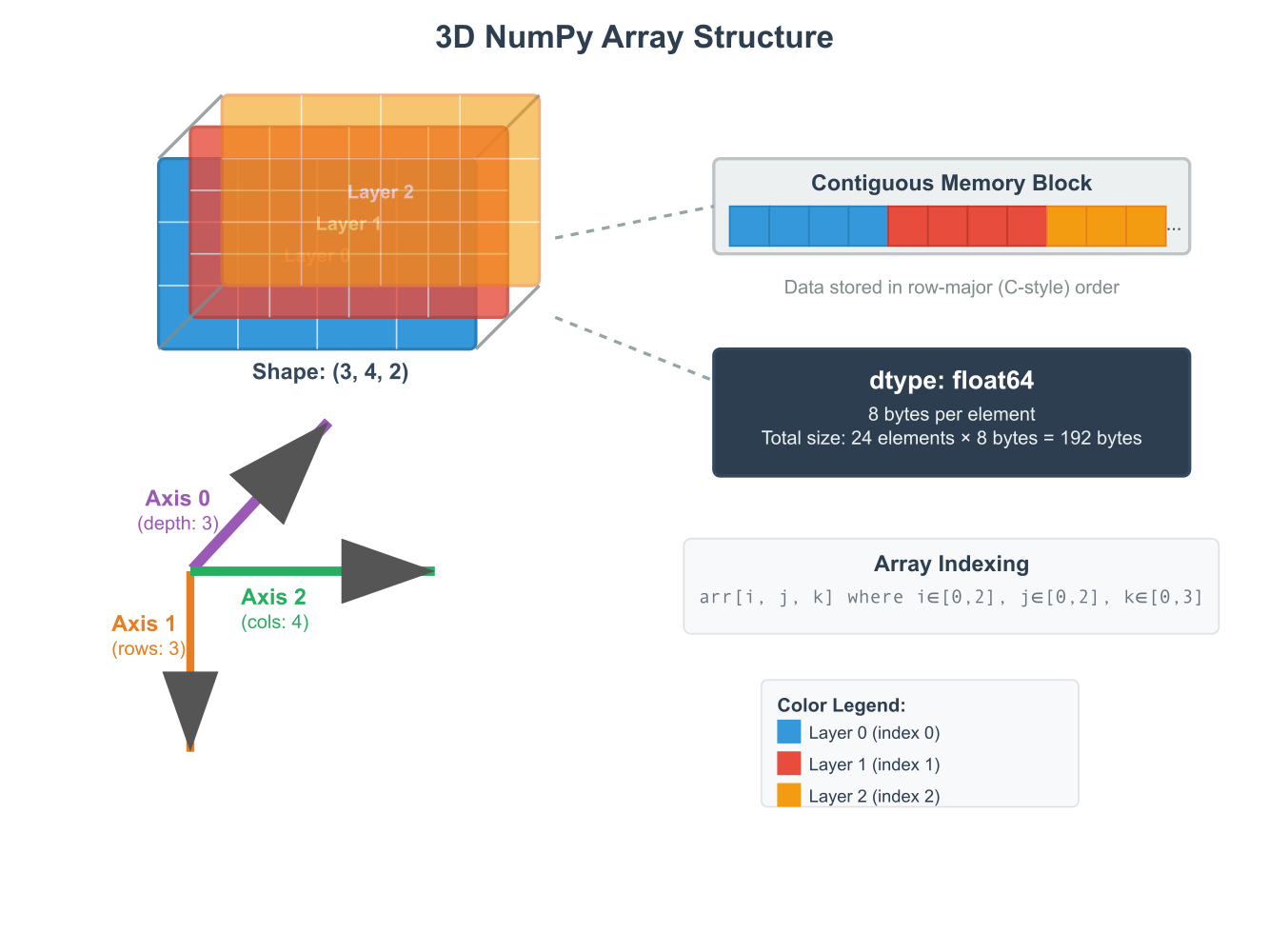
At the heart of the NumPy library lies the ndarray, or N-dimensional array. This object is a powerful data structure that serves as a multidimensional container for homogeneous data; that is, all elements within an array must be of the same data type. This constraint is a key differentiator from Python’s built-in lists and is fundamental to NumPy’s performance. By enforcing a single data type, NumPy can store the array’s data in a contiguous block of memory. This memory layout is crucial because it allows the underlying compiled C and Fortran code, upon which NumPy is built, to leverage modern CPU architectures for vectorized operations. When an operation is performed on a NumPy array, it is executed as a single, highly optimized instruction on the entire block of data (a process known as Single Instruction, Multiple Data or SIMD), rather than iterating through the elements one by one as a Python loop would. This is the essence of vectorization, a concept we will revisit throughout this chapter.
NumPy ndarray vs. Python List
| Feature | NumPy ndarray | Python List |
|---|---|---|
| Data Type | Homogeneous (all elements must be the same type, e.g., int64) | Heterogeneous (can contain mixed data types, e.g., integers, strings) |
| Memory Storage | Contiguous block of memory, highly efficient | Stores pointers to objects scattered in memory, less efficient |
| Performance | Fast, vectorized operations executed in compiled C code (SIMD) | Slow, operations require interpreted Python loops |
| Functionality | Optimized for numerical, scientific, and linear algebra operations | General-purpose, flexible container for storing items |
| Size | Fixed size upon creation | Dynamic size (can be easily appended to or resized) |
| Use Case | Large-scale numerical computation, machine learning, data analysis | General programming tasks, storing collections of items |
The ndarray object possesses several key attributes that describe its structure. The ndim attribute specifies the number of dimensions, or axes, of the array. The shape attribute is a tuple of integers indicating the size of the array along each dimension. For a matrix, the shape would be (rows, columns). The size attribute gives the total number of elements in the array, which is the product of the elements in the shape tuple. Finally, the dtype attribute is an object that describes the data type of the elements, such as int64, float32, or bool. Understanding these attributes is essential for debugging and manipulating arrays effectively. Mathematically, a 1D NumPy array can be seen as a vector, a 2D array as a matrix, and arrays with three or more dimensions as tensors. This direct mapping to fundamental mathematical objects is what makes NumPy such a natural and powerful tool for implementing machine learning algorithms, which are often expressed in the language of linear algebra.
Historical Development and Evolution
The genesis of NumPy can be traced back to the scientific computing community’s need for a high-performance numerical computing environment within Python. In the late 1990s, Python’s ease of use made it attractive, but its performance for numerical tasks was a significant bottleneck. The first major attempt to solve this was the Numeric library, developed by Jim Hugunin. Numeric introduced the array object and laid the groundwork for array-based computing in Python. Shortly after, another library called Numarray emerged, offering some improvements and a more flexible design. However, the existence of two competing libraries created fragmentation in the community.
In 2005, Travis Oliphant unified the best features of Numeric and Numarray into a single, powerful library: NumPy. This unification was a pivotal moment for scientific computing in Python. NumPy provided not only a fast and memory-efficient ndarray object but also a rich ecosystem of mathematical functions to operate on these arrays. It established a standard for array computing that other libraries could build upon, fostering the development of the rich scientific Python stack we know today. The design of NumPy was heavily influenced by the MATLAB programming language, aiming to provide a similarly expressive and high-performance environment for numerical analysis, but with the added benefits of being a free, open-source library integrated into a powerful general-purpose programming language. The introduction of concepts like broadcasting was a significant innovation, allowing for more intuitive and memory-efficient operations between arrays of different shapes, a feature that has become a cornerstone of modern numerical frameworks.
The Power of Vectorization and Broadcasting
Understanding Vectorization
Vectorization is the process of applying an operation to an entire array at once, rather than element by element. This is the core principle behind NumPy’s performance. When you write c = a + b, where a and b are NumPy arrays, you are not executing a Python loop. Instead, NumPy calls a pre-compiled, highly optimized C function that performs the element-wise addition directly in machine code. This approach has two primary benefits. First, it dramatically reduces the overhead associated with Python’s interpreted loops. Python is a dynamically typed language, and for each iteration of a loop, the interpreter must perform type checks and other bookkeeping, which adds significant computational cost. The C code in NumPy, by contrast, operates on a known, fixed data type, eliminating this overhead.
Second, vectorized operations can take advantage of modern CPU features like SIMD (Single Instruction, Multiple Data) vector processing units. These specialized hardware components can perform the same operation on multiple data points simultaneously. For example, a single instruction might add four pairs of floating-point numbers at once. When NumPy performs an element-wise operation on a large array stored in contiguous memory, it can feed chunks of this data directly to the SIMD units, achieving a level of parallelism that is impossible with a standard Python loop. The practical implication for an AI engineer is profound: code that is not only more concise and readable (e.g., a + b instead of a for loop) but also orders of magnitude faster. Mastering vectorization means thinking in terms of whole-array operations, a paradigm shift that is essential for efficient machine learning development.
graph LR
        subgraph Fast Path: NumPy Vectorization
            direction LR
            A2["NumPy Array 'a'<br>(Contiguous Memory)"] --> C2["Single C Operation<br><b>c = a + b</b><br><i>(SIMD Instruction)</i>"];
            B2["NumPy Array 'b'<br>(Contiguous Memory)"] --> C2;
            C2 --> R2[Result Array 'c'];
        end
        subgraph Slow Path: Python For-Loop
            direction LR
            A1[List 'a'] --> L1{For each element...};
            B1[List 'b'] --> L1;
            L1 --> P1["Python Interpreter<br><i>(Type Check, Overhead)</i>"];
            P1 --> C1[Add element 'i'];
            C1 --> L2{Append to new list};
            L2 --> L1;
            L2 --> R1[Result List 'c'];
        end


        style A1 fill:#9b59b6,stroke:#9b59b6,stroke-width:2px,color:#ebf5ee
        style B1 fill:#9b59b6,stroke:#9b59b6,stroke-width:2px,color:#ebf5ee
        style R1 fill:#2d7a3d,stroke:#2d7a3d,stroke-width:2px,color:#ebf5ee
        style L1 fill:#f39c12,stroke:#f39c12,stroke-width:1px,color:#283044
        style P1 fill:#f1c40f,stroke:#f1c40f,stroke-width:1px,color:#283044
        style C1 fill:#78a1bb,stroke:#78a1bb,stroke-width:1px,color:#283044
        style L2 fill:#78a1bb,stroke:#78a1bb,stroke-width:1px,color:#283044

        style A2 fill:#9b59b6,stroke:#9b59b6,stroke-width:2px,color:#ebf5ee
        style B2 fill:#9b59b6,stroke:#9b59b6,stroke-width:2px,color:#ebf5ee
        style C2 fill:#283044,stroke:#283044,stroke-width:2px,color:#ebf5ee
        style R2 fill:#2d7a3d,stroke:#2d7a3d,stroke-width:2px,color:#ebf5ee
The Rules of Broadcasting
Broadcasting is one of NumPy’s most powerful and sometimes misunderstood features. It describes how NumPy treats arrays with different shapes during arithmetic operations. In short, subject to certain constraints, the smaller array is “broadcast” across the larger array so that they have compatible shapes. This allows for element-wise operations to be performed without making explicit copies of the smaller array, leading to highly efficient computations both in terms of speed and memory. The rules of broadcasting are simple but their application is profound.
NumPy compares the shapes of the two arrays element-wise, starting from the trailing (rightmost) dimensions. Two dimensions are compatible if:
- They are equal.
- One of them is 1.
If these conditions are not met, a ValueError: operands could not be broadcast together exception is thrown. If the number of dimensions of the two arrays is different, the shape of the one with fewer dimensions is padded with ones on its leading (left) side. Let’s consider an example: adding a 1D array (vector) to a 2D array (matrix). Suppose we have a matrix A with shape (3, 4) and a vector v with shape (4,). To add them, NumPy compares their shapes. First, it aligns them to the right:
A.shape:(3, 4)v.shape:( , 4)
The trailing dimensions are both 4, so they are compatible. Now, NumPy looks at the next dimension. A has a dimension of size 3, while v has no corresponding dimension. NumPy prepends a 1 to v‘s shape, making it (1, 4). Now the shapes are:
A.shape:(3, 4)v.shape:(1, 4)
Comparing the dimensions again:
- Trailing dimension: 4 and 4 are equal.
- Leading dimension: 3 and 1 are compatible because one of them is 1.
Since all dimensions are compatible, broadcasting can proceed. NumPy will virtually “stretch” or “duplicate” the vector v along the dimension of size 1, three times, to match the shape of A. The addition is then performed element-wise. This mechanism is fundamental in machine learning, for instance, when adding a bias vector to the output of a matrix multiplication for every instance in a batch.

Advanced Array Manipulation
Advanced Indexing Techniques
Beyond basic slicing, NumPy offers more sophisticated indexing techniques that unlock powerful data manipulation capabilities. These are broadly categorized into integer array indexing and boolean array indexing. These methods allow for the selection of arbitrary elements from an array based on their position or condition, and importantly, they always return a copy of the data, not a view.
Integer array indexing allows you to construct a new array by selecting elements using another array of integers. For example, if you have a 1D array x and an index array i = np.array([1, 5, 3]), then x[i] will return a new array containing the elements at indices 1, 5, and 3 of x. This concept extends to multiple dimensions. If you have a 2D array A and provide two integer arrays, rows and cols, A[rows, cols] will return a 1D array containing the elements at the coordinates (rows[0], cols[0]), (rows[1], cols[1]), and so on. This is incredibly useful for quickly reordering or selecting specific, non-contiguous elements from a larger dataset. For instance, in a dataset of user profiles, you could use integer array indexing to fetch a specific subset of users in a particular order for analysis.
Boolean array indexing, on the other hand, allows you to select elements from an array based on a boolean condition. When you apply a comparison operator to a NumPy array (e.g., A > 5), it performs an element-wise comparison and returns a new boolean array of the same shape, with True where the condition is met and False otherwise. This boolean array can then be used as an index for the original array. The expression A[A > 5] will return a 1D array containing only the elements from A that are greater than 5. This technique is one of the most common and powerful ways to filter data in NumPy. It’s the foundation for many data cleaning and preprocessing tasks, such as removing outliers, replacing specific values, or selecting data points that meet a certain criterion, all without writing explicit Python loops.
Reshaping and Transposing Arrays
Manipulating the shape and orientation of arrays is a fundamental operation in data science and machine learning. NumPy provides a rich set of functions for this purpose, with reshape and transpose (or the .T attribute) being the most common. The reshape function allows you to change the shape of an array without changing its data, as long as the new shape is compatible with the original size. For example, a 1D array of 12 elements can be reshaped into a (3, 4) matrix or a (2, 6) matrix. A special value of -1 can be used in one dimension, and NumPy will automatically infer the correct size for that dimension. This is particularly useful in machine learning pipelines, for example, when preparing a flattened image vector to be fed into a fully connected neural network layer that expects a specific 2D input shape (batch size, number of features).
The transpose operation, accessed via the .T attribute or the np.transpose() function, permutes the dimensions of an array. For a 2D array (a matrix), this is the familiar operation of swapping rows and columns. Mathematically, it turns a matrix A of shape (m,n) into AT of shape (n,m). This is a cornerstone of linear algebra and is used constantly in machine learning algorithms. For example, the weight update rule in linear regression involves the transpose of the feature matrix. For higher-dimensional arrays (tensors), the transpose function can be given an axes argument, a tuple of integers specifying the new order of the dimensions. This provides fine-grained control over how the tensor is reoriented, a critical capability for operations in deep learning frameworks like TensorFlow and PyTorch, where the order of dimensions (e.g., batch, height, width, channels) can be significant. It’s important to note that both reshape and .T often return a view of the original array’s data whenever possible, meaning they don’t copy the underlying data. This makes them extremely fast and memory-efficient operations.
Practical Examples and Implementation
Mathematical Concept Implementation
Let’s translate the core mathematical concepts of vectors and matrices into NumPy code. The foundation of linear algebra is built upon these objects, and NumPy provides a direct and intuitive way to work with them.
A vector can be represented as a 1D NumPy array, and a matrix as a 2D array. We can perform fundamental operations like vector addition, scalar multiplication, and the dot product, which are central to almost every machine learning algorithm.
import numpy as np

# --- Vector Operations ---
# Create two vectors (1D arrays)
v1 = np.array([1, 2, 3])
v2 = np.array([4, 5, 6])
print(f"Vector v1: {v1}")
print(f"Vector v2: {v2}")

# Vector addition (element-wise)
v_sum = v1 + v2
print(f"Vector Sum (v1 + v2): {v_sum}")

# Scalar multiplication
v_scaled = v1 * 3
print(f"Scalar Multiplication (v1 * 3): {v_scaled}")

# Dot product of two vectors
# This is a fundamental operation in ML, e.g., for calculating the output of a neuron.
dot_product = np.dot(v1, v2)
# An alternative syntax is using the @ operator (preferred for Python 3.5+)
dot_product_alt = v1 @ v2
print(f"Dot Product (v1 . v2): {dot_product}")
print(f"Dot Product (v1 @ v2): {dot_product_alt}")


# --- Matrix Operations ---
# Create two matrices (2D arrays)
A = np.array([[1, 2], [3, 4]])
B = np.array([[5, 6], [7, 8]])
print(f"\nMatrix A:\n{A}")
print(f"Matrix B:\n{B}")

# Matrix addition (element-wise)
# Note: This requires matrices to have the same shape.
M_sum = A + B
print(f"Matrix Sum (A + B):\n{M_sum}")

# Element-wise multiplication (Hadamard Product)
# This is NOT matrix multiplication.
hadamard_product = A * B
print(f"Element-wise Product (A * B):\n{hadamard_product}")

# Matrix multiplication (Dot product for matrices)
# The number of columns in the first matrix must equal the number of rows in the second.
matrix_product = np.dot(A, B)
# Using the @ operator is more idiomatic for matrix multiplication
matrix_product_alt = A @ B
print(f"Matrix Product (A @ B):\n{matrix_product_alt}")

# Transpose of a matrix
A_T = A.T
print(f"Transpose of A:\n{A_T}")
Output:
Vector v1: [1 2 3]
Vector v2: [4 5 6]
Vector Sum (v1 + v2): [5 7 9]
Scalar Multiplication (v1 * 3): [3 6 9]
Dot Product (v1 . v2): 32
Dot Product (v1 @ v2): 32

Matrix A:
[[1 2]
 [3 4]]
Matrix B:
[[5 6]
 [7 8]]
Matrix Sum (A + B):
[[ 6  8]
 [10 12]]
Element-wise Product (A * B):
[[ 5 12]
 [21 32]]
Matrix Product (A @ B):
[[19 22]
 [43 50]]
Transpose of A:
[[1 3]
 [2 4]]
This code demonstrates how NumPy’s syntax closely mirrors mathematical notation, making it easy to translate formulas from papers and textbooks directly into efficient, working code. The use of operators like +, *, and @ for vectorized operations is a key feature that leads to clean and readable implementations.
AI/ML Application Examples
Broadcasting is not just a theoretical concept; it is used constantly in practical machine learning workflows. A classic example is standardizing features in a dataset. Feature scaling, such as Z-score normalization, is a common preprocessing step where you subtract the mean and divide by the standard deviation for each feature. This ensures that all features have a mean of 0 and a standard deviation of 1, which can significantly improve the performance of many algorithms like gradient descent.
Let’s see how broadcasting makes this trivial. Imagine we have a dataset of 100 samples and 5 features, represented as a (100, 5) matrix.
import numpy as np

# --- Vector Operations ---
# Create two vectors (1D arrays)
v1 = np.array([1, 2, 3])
v2 = np.array([4, 5, 6])
print(f"Vector v1: {v1}")
print(f"Vector v2: {v2}")

# Vector addition (element-wise)
v_sum = v1 + v2
print(f"Vector Sum (v1 + v2): {v_sum}")

# Scalar multiplication
v_scaled = v1 * 3
print(f"Scalar Multiplication (v1 * 3): {v_scaled}")

# Dot product of two vectors
# This is a fundamental operation in ML, e.g., for calculating the output of a neuron.
dot_product = np.dot(v1, v2)
# An alternative syntax is using the @ operator (preferred for Python 3.5+)
dot_product_alt = v1 @ v2
print(f"Dot Product (v1 . v2): {dot_product}")
print(f"Dot Product (v1 @ v2): {dot_product_alt}")


# --- Matrix Operations ---
# Create two matrices (2D arrays)
A = np.array([[1, 2], [3, 4]])
B = np.array([[5, 6], [7, 8]])
print(f"\nMatrix A:\n{A}")
print(f"Matrix B:\n{B}")

# Matrix addition (element-wise)
# Note: This requires matrices to have the same shape.
M_sum = A + B
print(f"Matrix Sum (A + B):\n{M_sum}")

# Element-wise multiplication (Hadamard Product)
# This is NOT matrix multiplication.
hadamard_product = A * B
print(f"Element-wise Product (A * B):\n{hadamard_product}")

# Matrix multiplication (Dot product for matrices)
# The number of columns in the first matrix must equal the number of rows in the second.
matrix_product = np.dot(A, B)
# Using the @ operator is more idiomatic for matrix multiplication
matrix_product_alt = A @ B
print(f"Matrix Product (A @ B):\n{matrix_product_alt}")

# Transpose of a matrix
A_T = A.T
print(f"Transpose of A:\n{A_T}")

# Generate some sample data (e.g., 100 people, 5 features like age, height, etc.)
np.random.seed(42)
X = np.random.rand(100, 5) * np.array([50, 100, 20, 5, 1]) + np.array([20, 150, 60, 1, 0])

print(f"Original data shape: {X.shape}")
print(f"First 5 rows of original data:\n{X[:5]}")

# 1. Calculate the mean of each feature (column)
# axis=0 computes the mean along the rows for each column
mean = np.mean(X, axis=0)
print(f"\nMean of each feature (shape {mean.shape}):\n{mean}")

# 2. Calculate the standard deviation of each feature
std_dev = np.std(X, axis=0)
print(f"Std Dev of each feature (shape {std_dev.shape}):\n{std_dev}")

# 3. Standardize the data using broadcasting
# X is (100, 5)
# mean is (5,)
# std_dev is (5,)
# NumPy broadcasts `mean` and `std_dev` to match the shape of X
X_scaled = (X - mean) / std_dev

print(f"\nScaled data shape: {X_scaled.shape}")
print(f"First 5 rows of scaled data:\n{X_scaled[:5]}")

# Verify the result
print(f"\nMean of scaled data (should be close to 0):\n{np.mean(X_scaled, axis=0)}")
print(f"Std Dev of scaled data (should be close to 1):\n{np.std(X_scaled, axis=0)}")
Outputs:
Vector v1: [1 2 3]
Vector v2: [4 5 6]
Vector Sum (v1 + v2): [5 7 9]
Scalar Multiplication (v1 * 3): [3 6 9]
Dot Product (v1 . v2): 32
Dot Product (v1 @ v2): 32

Matrix A:
[[1 2]
 [3 4]]
Matrix B:
[[5 6]
 [7 8]]
Matrix Sum (A + B):
[[ 6  8]
 [10 12]]
Element-wise Product (A * B):
[[ 5 12]
 [21 32]]
Matrix Product (A @ B):
[[19 22]
 [43 50]]
Transpose of A:
[[1 3]
 [2 4]]
Original data shape: (100, 5)
First 5 rows of original data:
[[3.87270059e+01 2.45071431e+02 7.46398788e+01 3.99329242e+00
  1.56018640e-01]
 [2.77997260e+01 1.55808361e+02 7.73235229e+01 4.00557506e+00
  7.08072578e-01]
 [2.10292247e+01 2.46990985e+02 7.66488528e+01 2.06169555e+00
  1.81824967e-01]
 [2.91702255e+01 1.80424224e+02 7.04951286e+01 3.15972509e+00
  2.91229140e-01]
 [5.05926447e+01 1.63949386e+02 6.58428930e+01 2.83180922e+00
  4.56069984e-01]]

Mean of each feature (shape (5,)):
[ 45.23553529 202.52323262  69.75395932   3.60627075   0.45391341]
Std Dev of each feature (shape (5,)):
[14.79858181 29.84016701  5.86686962  1.4587506   0.30658573]

Scaled data shape: (100, 5)
First 5 rows of scaled data:
[[-0.43980764  1.42586997  0.83279838  0.26531037 -0.97165243]
 [-1.17820812 -1.56550301  1.29022189  0.27373034  0.82899867]
 [-1.63571827  1.49019785  1.17522528 -1.05883432 -0.88747915]
 [-1.08559793 -0.74057924  0.12633131 -0.30611515 -0.53063223]
 [ 0.36200154 -1.29268199 -0.66663598 -0.53090743  0.00703416]]

Mean of scaled data (should be close to 0):
[ 3.18634008e-16  1.67088565e-15 -3.13971071e-15 -1.48769885e-16
  6.94999613e-16]
Std Dev of scaled data (should be close to 1):
[1. 1. 1. 1. 1.]
Without broadcasting, we would have to write a loop to iterate over each feature (column) or tile the mean and std_dev vectors to match the shape of X, which is far less efficient and harder to read. Broadcasting allows us to express the mathematical formula X_scaled=fracX−musigma directly and elegantly in code.
Visualization and Interactive Examples
Visualizing mathematical concepts can greatly aid understanding. Let’s visualize the effect of broadcasting. We’ll take a 1D array (a ramp of values) and add it to a 1D column vector (another ramp). Broadcasting will turn this into a 2D grid. We can use Matplotlib to visualize the resulting 2D array as an image.
import matplotlib.pyplot as plt

# Create a 1D row vector (shape (10,))
a = np.arange(0, 10, 1)
print(f"Shape of a: {a.shape}")
print(f"a: {a}")

# Create a 1D column vector. We need to reshape it to (10, 1)
b = np.arange(0, 10, 1).reshape(10, 1)
# An alternative is using np.newaxis
# b = np.arange(0, 10, 1)[:, np.newaxis]
print(f"\nShape of b: {b.shape}")
print(f"b:\n{b}")

# Add them together. Broadcasting will be applied.
# a (10,) will be treated as (1, 10)
# b is (10, 1)
# The result will be a (10, 10) matrix
c = a + b
print(f"\nShape of c: {c.shape}")
print(f"Result c:\n{c}")

# Visualize the result
plt.figure(figsize=(8, 6))
plt.imshow(c, cmap='viridis', interpolation='nearest')
plt.colorbar(label='Value')
plt.title('Visualization of Broadcasting: (1, 10) + (10, 1) -> (10, 10)')
plt.xlabel('Dimension from vector a')
plt.ylabel('Dimension from vector b')
plt.show()
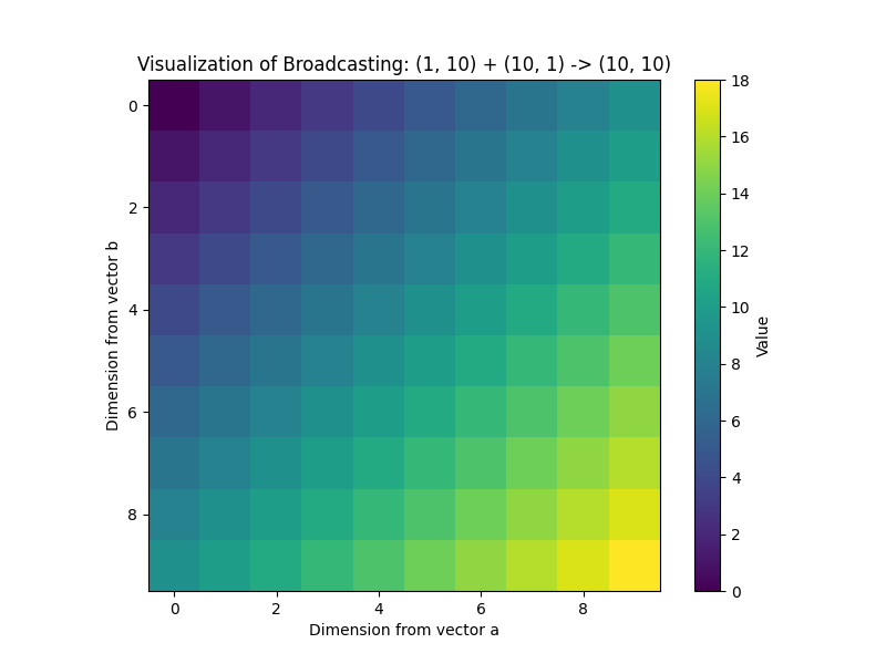
This visualization clearly shows how the row vector a was “stretched” vertically and the column vector b was “stretched” horizontally to fill a 10×10 grid, where each cell c[i, j] is the sum of a[j] and b[i]. This simple example illustrates a powerful technique used in generating coordinate grids, computing distance matrices, and many other applications in scientific computing.
Computational Exercises
Let’s reinforce our understanding with a hands-on exercise: implementing a function to calculate the pairwise Euclidean distance between two sets of points. This is a common task in clustering algorithms (like K-Means) and classification (like K-Nearest Neighbors).
Given two arrays, A of shape (M, D) and B of shape (N, D), where M and N are the number of points and D is the number of dimensions, we want to compute a distance matrix D of shape (M, N) where D[i, j] is the Euclidean distance between the i-th point in A and the j-th point in B.
The formula for the squared Euclidean distance is: $$d(x, y)^2 = \sum_{k=1}^{D} (x_k – y_k)^2 = \|x-y\|^2$$. This can be expanded to: $$\|x\|^2 – 2x \cdot y + \|y\|^2$$. We can compute this for all pairs of points efficiently using vectorization and broadcasting.
def pairwise_distance(A, B):
    """
    Computes the pairwise Euclidean distance matrix between two sets of points.

    Args:
        A (np.ndarray): A matrix of shape (M, D)
        B (np.ndarray): A matrix of shape (N, D)

    Returns:
        np.ndarray: A matrix of shape (M, N) where D[i, j] is the distance
                    between A[i] and B[j].
    """
    # Number of points
    M = A.shape[0]
    N = B.shape[0]

    # Calculate the squared norm of each point in A and B
    # (M, 1) array
    A_squared_norms = np.sum(A**2, axis=1).reshape(M, 1)
    # (N,) array
    B_squared_norms = np.sum(B**2, axis=1)

    # Calculate the dot product term
    # (M, D) @ (D, N) -> (M, N)
    dot_product = A @ B.T

    # Use broadcasting to compute the squared distances
    # A_squared_norms (M, 1) is broadcast across N columns
    # B_squared_norms (N,) is broadcast across M rows
    # dot_product is (M, N)
    squared_distances = A_squared_norms - 2 * dot_product + B_squared_norms

    # The distances may be slightly negative due to floating point inaccuracies.
    # Clip at 0 before taking the square root.
    squared_distances = np.maximum(squared_distances, 0)

    return np.sqrt(squared_distances)

# --- Example Usage ---
np.random.seed(0)
points_A = np.random.rand(3, 2) # 3 points in 2D
points_B = np.random.rand(4, 2) # 4 points in 2D

print("Points A:\n", points_A)
print("\nPoints B:\n", points_B)

# Calculate the distance matrix
dist_matrix = pairwise_distance(points_A, points_B)
print("\nPairwise Distance Matrix (shape 3x4):\n", dist_matrix)

# Verification: Manually calculate distance between A[0] and B[0]
manual_dist = np.sqrt(np.sum((points_A[0] - points_B[0])**2))
print(f"\nManual distance between A[0] and B[0]: {manual_dist}")
print(f"Matrix distance between A[0] and B[0]: {dist_matrix[0, 0]}")
assert np.isclose(manual_dist, dist_matrix[0, 0])
Outputs:
Points A:
 [[0.5488135  0.71518937]
 [0.60276338 0.54488318]
 [0.4236548  0.64589411]]

Points B:
 [[0.43758721 0.891773  ]
 [0.96366276 0.38344152]
 [0.79172504 0.52889492]
 [0.56804456 0.92559664]]

Pairwise Distance Matrix (shape 3x4):
 [[0.20869372 0.53118409 0.30612356 0.2112843 ]
 [0.3842079  0.39536284 0.18963685 0.38229325]
 [0.2462733  0.60040816 0.38621822 0.31477278]]

Manual distance between A[0] and B[0]: 0.20869371845180915
Matrix distance between A[0] and B[0]: 0.208693718451809
This exercise shows how a complex mathematical operation can be broken down into vectorized steps. By calculating the norms and dot products separately and then combining them using broadcasting, we avoid any explicit loops over the points, resulting in a highly efficient implementation that scales well to large datasets.
Real-World Problem Applications
Advanced indexing is crucial for tasks like image manipulation in computer vision. For example, we might want to apply a color mask to an image, setting certain pixels to a specific color based on a condition.
Let’s take a sample image (represented as a 3D NumPy array: height, width, channels) and use boolean indexing to select all pixels that are “mostly blue” and change their color to bright yellow.
import numpy as np
import matplotlib.pyplot as plt

# We'll create a sample image with NumPy for demonstration
# In a real scenario, you would load an image using a library like Pillow or OpenCV
# Image shape: (height, width, channels) where channels are Red, Green, Blue
image = np.zeros((200, 300, 3), dtype=np.uint8)

# Create some blue-ish and red-ish regions
image[50:150, 50:150] = [10, 20, 180]   # A blue square
image[50:150, 200:250] = [200, 30, 40] # A red square
image += np.random.randint(0, 20, size=image.shape, dtype=np.uint8) # Add some noise

# Define the condition for "mostly blue"
# We'll select pixels where the blue channel is much larger than red and green
blue_channel = image[:, :, 2]
red_channel = image[:, :, 0]
green_channel = image[:, :, 1]

# Create a boolean mask
# The '&' operator performs element-wise logical AND
is_blue_mask = (blue_channel > 150) & (red_channel < 50) & (green_channel < 50)

# The mask is a 2D array of booleans (height, width)
print(f"Shape of the boolean mask: {is_blue_mask.shape}")

# Use the boolean mask to change the color of the selected pixels
# We are indexing a (200, 300, 3) array with a (200, 300) mask.
# NumPy applies the mask across all 3 color channels.
image_copy = image.copy()
image_copy[is_blue_mask] = [255, 255, 0] # Set to bright yellow (R=255, G=255, B=0)

# Display the original and modified images
fig, axes = plt.subplots(1, 2, figsize=(12, 6))
axes[0].imshow(image)
axes[0].set_title("Original Image")
axes[0].axis('off')

axes[1].imshow(image_copy)
axes[1].set_title("Modified Image (Blue replaced with Yellow)")
axes[1].axis('off')

plt.show()
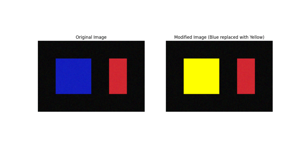
This example demonstrates the power and expressiveness of boolean indexing. The complex logic of finding and modifying specific pixels is condensed into a few clear, vectorized lines of code. This is far more efficient and less error-prone than iterating through every pixel with nested loops. This exact technique is used in applications ranging from simple color filtering to creating masks for object segmentation in advanced computer vision models.
Industry Applications and Case Studies
NumPy’s role as the foundational library for numerical computing in Python makes it ubiquitous across industries that leverage data for decision-making. Its applications are not confined to a single domain but are a fundamental component of the entire AI and data science workflow.
- Financial Modeling and Algorithmic Trading: In the world of quantitative finance, speed is paramount. Hedge funds and investment banks use NumPy to analyze vast amounts of time-series data, model asset prices, and backtest trading strategies. Operations like calculating moving averages, portfolio volatility (requiring matrix multiplication on covariance matrices), and running Monte Carlo simulations are all performed using NumPy’s vectorized functions. The ability to perform complex calculations on entire arrays of stock prices or economic indicators in milliseconds is a critical competitive advantage. The challenge here is processing streaming data with extremely low latency, and NumPy’s C-backend provides the necessary performance without having to leave the flexible Python environment.
- Climate Science and Environmental Modeling: Researchers analyzing climate data from satellites and weather stations rely on NumPy to process massive, multi-dimensional datasets (e.g., temperature, pressure, humidity over a 3D grid of latitude, longitude, and altitude). NumPy is used to perform spatial and temporal aggregations, apply mathematical models to forecast weather patterns, and analyze long-term climate trends. Broadcasting is particularly useful for applying calibration constants or atmospheric models across large grids of sensor data. The business impact relates to agriculture, disaster prediction, and resource management, where accurate and timely analysis of environmental data is crucial.
- Computational Biology and Genomics: The analysis of genomic data involves manipulating enormous matrices where rows might represent genes and columns represent samples. NumPy is used for tasks like identifying genetic markers, performing statistical tests on gene expression levels, and clustering patients based on their genetic profiles. Advanced indexing is used to filter and select specific genes or patient cohorts for analysis. The performance of NumPy is critical for handling datasets that can easily run into terabytes, enabling researchers to accelerate the discovery of new drugs and personalized medical treatments.
- Image and Signal Processing in Aerospace: Aerospace and defense companies use NumPy extensively for processing signals from radar, sonar, and satellite imagery. These applications involve applying filters (convolutions), performing Fourier transforms to analyze frequency components, and cleaning noise from sensor data. These are all array-intensive operations where NumPy’s performance is essential. For example, in satellite imaging, NumPy arrays are used to represent images, and boolean indexing is used to mask clouds or other artifacts before analysis. The technical challenge is often real-time processing, and NumPy’s efficiency makes it a cornerstone of these systems.
Best Practices and Common Pitfalls
While NumPy is incredibly powerful, using it effectively requires an understanding of its design principles and potential pitfalls. Adhering to best practices ensures that your code is not only fast but also memory-efficient, readable, and maintainable.
- Embrace Vectorization, Avoid Loops: The single most important best practice is to think in terms of whole-array operations. If you find yourself writing a
forloop that iterates over the elements of a NumPy array, pause and search for a vectorized alternative. NumPy has a vast library of “universal functions” (ufuncs) that can perform almost any element-wise operation. Using functions likenp.sum,np.mean,np.exp, or comparison operators directly on arrays will always be significantly faster than a manual loop. - Understand Views vs. Copies: This is a common source of bugs for new users. Many NumPy operations, such as basic slicing (
arr[1:5]) or reshaping, return a view of the original array’s data. This means the new array object points to the same underlying memory. Modifying the view will modify the original array. Other operations, like advanced indexing (arr[[1, 5]]) or arithmetic operations, return a copy. Be mindful of this distinction. If you need to ensure you are not modifying the original data, explicitly use the.copy()method.Warning: Unintentionally modifying an array through a view can lead to subtle and hard-to-debug errors, especially in complex data processing pipelines. - Leverage Broadcasting Wisely: Broadcasting is a powerful tool for writing clean and efficient code, but it can also consume a large amount of memory if not used carefully. When you broadcast a small array to a very large one, NumPy doesn’t actually create a massive copy in memory, but the intermediate results of operations can. Be aware of the shapes of your arrays and how they will interact. Sometimes, it may be more memory-efficient to iterate in chunks if broadcasting would create an unmanageably large intermediate array.
- Choose the Right Data Type (
dtype): NumPy arrays have a fixed data type. Choosing the appropriatedtypecan have a significant impact on memory usage and performance. If you are working with integer data that will never exceed a certain value, usingnp.int32ornp.int16instead of the defaultnp.int64can halve your memory footprint. Similarly, if single-precision floating-point numbers (np.float32) are sufficient for your calculations, use them instead of double-precision (np.float64). This is particularly important when working with very large datasets or on memory-constrained hardware like GPUs. - Pre-allocate Arrays: Python lists can grow dynamically, but NumPy arrays have a fixed size upon creation. Repeatedly appending to a NumPy array using functions like
np.appendis highly inefficient because it involves creating a new, larger array and copying all the old data over in each step. If you know the final size of your array, it is far more efficient to pre-allocate an empty array of that size and then fill in the values.
Hands-on Exercises
These exercises are designed to build upon the concepts covered in the chapter, progressing from fundamental operations to a more complex, applied problem.
- Vector and Matrix Operations Practice:
- Objective: Reinforce your understanding of basic linear algebra operations in NumPy.
- Task: Create a 3×3 matrix
Aand a 3-element vectorb.- Calculate the matrix-vector product
c = Ab. - Calculate the dot product of vector
bwith itself. - Create another 3×3 matrix
Band compute the matrix productD = AB. - Compute the element-wise product of
AandB.
- Calculate the matrix-vector product
- Verification: Manually compute the first element of
candDto verify your results. Check the shapes of all resulting arrays.
- Broadcasting for Data Normalization:
- Objective: Apply broadcasting to a practical data preprocessing task.
- Task: Create a random 10×4 matrix representing a dataset with 10 samples and 4 features.
- For each feature (column), find the minimum and maximum values.
- Using these min/max values and broadcasting, perform min-max normalization on the dataset. The formula is: Xnorm=X−XminXmax−XminXnorm=Xmax−XminX−Xmin.
- Verification: After normalization, the minimum value in each column should be 0 and the maximum value should be 1. Use
np.minandnp.maxwithaxis=0to confirm this.
- Filtering with Boolean Indexing:
- Objective: Use boolean indexing to filter and analyze a dataset.
- Task: Create a 1D NumPy array of 1000 random integers between 0 and 500.
- Create a boolean mask to identify all numbers that are greater than 400.
- Use the mask to select these numbers. How many are there?
- In a single line of code, calculate the mean of all numbers in the original array that are less than or equal to 100.
- Create a new array where all values greater than 250 are replaced with the value -1.
- Verification: Check the length of the filtered array from step 2. Manually inspect the first few elements of the array from step 4 to ensure the replacement worked correctly.
- Team Activity: Implementing a Simple Image Filter:
- Objective: Apply array slicing and vectorized operations to implement a 2D convolution, the basis of image filtering.
- Task:
- Create a 10×10 grayscale image (a 2D NumPy array with random values between 0 and 255).
- Create a 3×3 kernel, for example, a simple blurring kernel:
kernel = np.ones((3, 3)) / 9.0. - Write a function that takes the image and kernel as input and returns the filtered image. Do not use libraries like
scipy.signal.convolve2d. Instead, use nested loops to iterate over the image pixels (excluding the border). For each pixel, extract the 3×3 neighborhood, perform an element-wise product with the kernel, and sum the result. This sum is the new pixel value. - Advanced Challenge: Can you vectorize this operation to avoid the inner loops over the kernel? (Hint: This is a very challenging problem that leads to advanced techniques like using
np.lib.stride_tricks). Discuss the performance difference between the looped and vectorized approaches.
- Verification: The output image should have a slightly blurred appearance compared to the noisy original. The output shape should be smaller than the input shape due to not processing the borders (e.g., an 8×8 output for a 10×10 input).
Tools and Technologies
The primary tool for this chapter is, of course, the NumPy library itself. It is the cornerstone of the scientific Python ecosystem.
- NumPy:
- Installation: NumPy is typically installed as part of a larger scientific distribution like Anaconda, but it can also be installed directly using Python’s package manager:
pip install numpy - Setup: In your Python scripts, the standard convention is to import NumPy with the alias
np:import numpy as np - Version: It is recommended to use a recent version of NumPy (e.g., 1.23+), as newer versions often include performance improvements and new features. You can check your version with
np.__version__.
- Installation: NumPy is typically installed as part of a larger scientific distribution like Anaconda, but it can also be installed directly using Python’s package manager:
- Jupyter Notebook / JupyterLab:
- Purpose: These are interactive development environments that are exceptionally well-suited for data analysis and numerical computation. They allow you to write and execute code in cells, interleave it with text and visualizations, and see the results immediately. This is ideal for exploring NumPy’s features and debugging array manipulations.
- Integration: Jupyter works seamlessly with NumPy and Matplotlib, making it the standard tool for interactive data science work.
- Matplotlib:
- Purpose: The de facto standard library for plotting and data visualization in Python. As seen in the examples, it is invaluable for visualizing NumPy arrays and understanding the effects of different operations.
- Installation:
pip install matplotlib
- Alternative Tools:
- While NumPy is the standard, it’s worth knowing about alternatives for specific use cases. CuPy is a GPU-accelerated library with a NumPy-compatible API, allowing you to speed up computations by running them on NVIDIA GPUs with minimal code changes. For distributed computing on massive datasets that don’t fit into a single machine’s memory, libraries like Dask can parallelize NumPy operations across a cluster of computers.
Summary
This chapter provided a deep dive into NumPy, the fundamental package for numerical computing in Python. We moved from basic principles to advanced applications, establishing the skills necessary for any AI engineering role.
- Key Concepts Learned:
- The NumPy
ndarrayis a memory-efficient, homogeneous data structure that enables high-performance vectorized operations. - Vectorization is the process of applying operations to entire arrays at once, which leverages compiled C code and modern CPU architectures to achieve massive speedups over Python loops.
- Broadcasting provides a powerful and efficient mechanism for performing arithmetic operations on arrays of different but compatible shapes without making explicit copies.
- Advanced indexing (integer and boolean) and shape manipulation (
reshape,.T) provide a flexible and powerful syntax for complex data selection and transformation tasks.
- The NumPy
- Major Achievements and Skills Gained:
- You can now implement mathematical formulas and algorithms directly and efficiently using NumPy’s array operations.
- You are equipped to write clean, performant, and Pythonic code for data preprocessing and manipulation, a critical step in any machine learning pipeline.
- You understand the crucial difference between array views and copies, enabling you to write safer and more memory-efficient code.
- Real-World Applicability:
- The skills learned in this chapter are directly applicable to virtually every domain of AI and data science, from finance and biology to computer vision and natural language processing. NumPy is the lingua franca of numerical data in Python, and mastering it is a prerequisite for effective work in the field. This foundation will be built upon in subsequent chapters as we use NumPy to implement machine learning algorithms from scratch.
Further Reading and Resources
- NumPy Official Documentation: The definitive source for all NumPy functions and concepts. The user guide and tutorials are excellent.
- “Python for Data Analysis, 3rd Edition” by Wes McKinney: Written by the creator of Pandas, this book has several excellent chapters on NumPy that are full of practical examples.
- “From Python to NumPy” by Nicolas P. Rougier: An open-access book that provides a deep and visually intuitive guide to thinking in a vectorized manner with NumPy.
- SciPy Lecture Notes: An excellent, community-created set of tutorials on the scientific Python ecosystem, with a strong focus on NumPy fundamentals.
- “A Visual Intro to NumPy and Data Representation” by Jay Alammar: An intuitive, blog-style introduction that is great for visual learners.
- “Elegant SciPy: The Art of Scientific Python” by Juan Nunez-Iglesias, Stéfan van der Walt, and Harriet Dashnow: This book showcases more advanced and elegant ways to use NumPy and other scientific libraries to solve real-world problems.
Glossary of Terms
ndarray: The core N-dimensional array object in NumPy. It is a container for homogeneous data with a fixed size and data type.- Vectorization: The process of rewriting loop-based, scalar-oriented code to use array-based operations, allowing for much faster execution.
- Broadcasting: A set of rules by which NumPy allows operations on arrays of different shapes. The smaller array is virtually “stretched” to match the shape of the larger array.
- Universal Function (ufunc): A function that operates on
ndarrays in an element-by-element fashion. Examples includenp.add,np.sin, andnp.exp. - Axis: A dimension of a NumPy array. For a 2D array, axis 0 represents the rows and axis 1 represents the columns.
- Shape: A tuple of integers that defines the size of the array along each dimension.
dtype: A NumPy object that describes the data type of the elements in an array (e.g.,int64,float32).- View: An array object that looks at the same memory buffer as another array. Modifying a view will affect the original array.
- Copy: A new array object with its own data. Modifications to a copy do not affect the original array.
- Advanced Indexing: The use of integer or boolean arrays to index another array, allowing for the selection of arbitrary elements. This always returns a copy.
Meta Description and SEO Tags
Meta Description: Master NumPy for AI and machine learning. This comprehensive chapter covers array operations, broadcasting, vectorization, and advanced indexing with practical Python examples.
SEO Tags: NumPy, Python, Machine Learning, Data Science, AI Engineering, Numerical Computing, Array Broadcasting, Vectorization, NumPy Tutorial, Python for AI, Data Manipulation, Scientific Computing
