
Chapter 16: Information Theory: Entropy, Cross-entropy, & KL Divergence
Chapter Objectives
Upon completing this chapter, you will be able to:
- Understand the foundational concepts of information theory, including information content (surprisal) and its relationship to probability.
- Analyze and calculate Shannon entropy for various probability distributions to quantify uncertainty.
- Implement cross-entropy as a loss function for classification models and explain its role in measuring the discrepancy between predicted and true distributions.
- Design and interpret machine learning experiments using Kullback-Leibler (KL) divergence to measure the difference between two probability distributions.
- Optimize model training by selecting appropriate information-theoretic loss functions and understanding their mathematical properties and numerical stability.
- Deploy these concepts to evaluate and compare generative models, analyze policy changes in reinforcement learning, and solve real-world problems in AI engineering.
Introduction
In the landscape of artificial intelligence, our primary goal is often to build models that can learn from data and make accurate predictions about the world. At the heart of this learning process lies a fundamental question: how do we quantify what a model knows and what it still needs to learn? How do we measure the “distance” between a model’s predictions and the ground truth it aims to capture? The answer, elegant and profound, comes from the field of information theory. Originally developed by Claude Shannon in the 1940s to optimize telecommunication systems, information theory provides a mathematical framework for quantifying information, uncertainty, and randomness.
This chapter delves into the core concepts of information theory that have become indispensable in modern AI engineering. We will explore entropy, a measure of the inherent uncertainty within a single probability distribution. We will then examine cross-entropy, which quantifies the inefficiency of using one probability distribution to represent another—a concept that forms the bedrock of most modern classification loss functions. Finally, we will investigate Kullback-Leibler (KL) divergence, a measure of how one probability distribution diverges from another, which is critical for training sophisticated generative models and in reinforcement learning. Understanding these principles is not merely an academic exercise; it is essential for designing effective loss functions, evaluating model performance, and grasping the theoretical underpinnings of why certain algorithms, from simple logistic regression to complex Variational Autoencoders (VAEs), work the way they do. This chapter will equip you with the theoretical knowledge and practical skills to wield these powerful tools in your own AI development work.
Technical Background
The journey into information theory begins with a simple, intuitive idea: events that are less likely to occur provide more information when they happen. An announcement that the sun will rise tomorrow morning contains very little new information because it is a near-certainty. However, an announcement of a surprise solar eclipse for tomorrow would contain a great deal of information. Information theory formalizes this intuition, providing a rigorous mathematical language to discuss and measure information. This framework is not just an abstract theory; it directly enables us to build and optimize machine learning models by defining what it means for a model’s predictions to be “close” to the truth.
Fundamental Concepts and Definitions
At its core, information theory is built upon the concepts of probability and surprise. The amount of information we gain from observing an event is directly related to how surprising that event is. This “surprise” is mathematically captured and forms the basis for the more complex ideas of entropy and divergence that are so crucial to machine learning.
Core Terminology and Mathematical Foundations
The foundational unit of information theory is information content, also known as surprisal. It is a measure of the surprise associated with a particular outcome. For an event \(x\) with probability \(P(x)\), its information content \(I(x)\) is defined as:\[I(x) = -\log_b(P(x)) = \log_b\left(\frac{1}{P(x)}\right)\]
The base of the logarithm, \(b\), determines the units of information. In computer science and machine learning, we almost always use base 2 (\(b=2\)), and the unit of information is the bit. If we use the natural logarithm (base \(e\)), the unit is the nat. The negative sign ensures that the information content is non-negative, since probabilities are between 0 and 1, and their logarithms are non-positive.
From this definition, we can see the inverse relationship between probability and information. A high-probability event (\(P(x) \to 1\)) has very low information content (\(I(x) \to 0\)), meaning it is not surprising. Conversely, a low-probability event (\(P(x) \to 0\)) has very high information content (\(I(x) \to \infty\)), signifying a great deal of surprise.
While information content applies to a single outcome, we are often interested in the average amount of information produced by a random variable over all its possible outcomes. This brings us to the concept of Shannon Entropy, denoted \(H(X)\). Entropy is the expected value of the information content of a random variable \(X\). For a discrete random variable \(X\) with possible outcomes \(x_1, x_2, \ldots, x_n\) and a probability mass function \(P(X)\), the entropy is calculated as:\[H(X) = \mathbb{E}[I(X)] = \sum_{i=1}^n P(x_i)I(x_i) = -\sum_{i=1}^n P(x_i)\log_2(P(x_i))\]
Entropy can be interpreted in several ways:
- Average Surprise: It is the average level of surprise we should expect from observing an outcome from the distribution.
- Measure of Uncertainty: It quantifies the uncertainty or randomness of a random variable. A distribution with high entropy is highly unpredictable, while one with low entropy is more deterministic.
- Optimal Compression: From a data compression perspective, \(H(X)\) represents the theoretical lower bound on the average number of bits required to encode a message drawn from the distribution \(P(X)\).
A uniform probability distribution (where all outcomes are equally likely) has the maximum possible entropy, as it represents the highest level of uncertainty. Conversely, a distribution where one outcome has a probability of 1 and all others have a probability of 0 has an entropy of 0, as there is no uncertainty about the outcome.
%%{ init: { 'theme': 'base', 'themeVariables': { 'fontFamily': 'Open Sans' } } }%%
graph LR
    subgraph "Low Entropy Distribution (Biased Coin)"
        direction LR
        L_Start(Start) --> L_Flip{Flip Coin}
        L_Flip --> L_Heads("Heads<br><b>P = 0.95</b>")
        L_Flip --> L_Tails("Tails<br>P = 0.05")
        L_Heads --> L_End([Outcome Known])
        L_Tails --> L_End
        A["Low uncertainty<br>Low <i>surprise</i><br><b>Low Entropy</b>"]
    end

    subgraph "High Entropy Distribution (Fair Coin)"
        direction LR
        H_Start(Start) --> H_Flip{Flip Coin}
        H_Flip --> H_Heads("Heads<br><b>P = 0.50</b>")
        H_Flip --> H_Tails("Tails<br><b>P = 0.50</b>")
        H_Heads --> H_End([Outcome Known])
        H_Tails --> H_End
        B[High uncertainty<br>High <i>surprise</i><br><b>High Entropy</b>]

    end

    style L_Start fill:#283044,stroke:#283044,stroke-width:2px,color:#ebf5ee
    style H_Start fill:#283044,stroke:#283044,stroke-width:2px,color:#ebf5ee
    style L_Flip fill:#f39c12,stroke:#f39c12,stroke-width:1px,color:#283044
    style H_Flip fill:#f39c12,stroke:#f39c12,stroke-width:1px,color:#283044
    style L_Heads fill:#78a1bb,stroke:#78a1bb,stroke-width:1px,color:#283044
    style L_Tails fill:#78a1bb,stroke:#78a1bb,stroke-width:1px,color:#283044
    style H_Heads fill:#78a1bb,stroke:#78a1bb,stroke-width:1px,color:#283044
    style H_Tails fill:#78a1bb,stroke:#78a1bb,stroke-width:1px,color:#283044
    style L_End fill:#2d7a3d,stroke:#2d7a3d,stroke-width:2px,color:#ebf5ee
    style H_End fill:#2d7a3d,stroke:#2d7a3d,stroke-width:2px,color:#ebf5ee
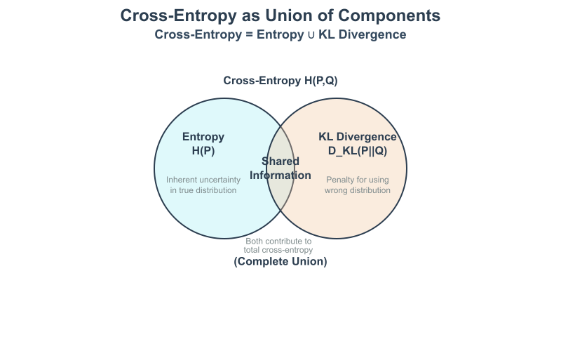
The Relationship Between Entropy, Cross-Entropy, and KL Divergence
These three concepts are deeply interconnected. While entropy measures the uncertainty of a single distribution, cross-entropy and KL divergence involve comparing two different distributions. Let’s consider two discrete probability distributions, \(P\) and \(Q\), over the same set of events \(\mathcal{X}\).
Cross-Entropy (\(H(P, Q)\)) arises from a practical question in coding theory: what is the average number of bits needed to encode events from a true distribution \(P\) if we use an encoding scheme optimized for a different, estimated distribution \(Q\)? Its formula is:\[H(P,Q) = -\sum_{x \in \mathcal{X}} P(x)\log_2(Q(x))\]
Notice the similarity to the entropy formula. Here, we are weighting the information content of the outcomes from \(Q\) (\(-\log_2(Q(x))\)) by the true probabilities from \(P\). Cross-entropy is not symmetric, meaning \(H(P, Q) \neq H(Q, P)\) in general. In machine learning, \(P\) is typically the true data distribution (e.g., the one-hot encoded labels in a classification problem), and \(Q\) is the model’s predicted probability distribution. Minimizing the cross-entropy loss during training, therefore, means making the model’s predictions \(Q\) as close as possible to the true distribution \(P\).
This leads us to Kullback-Leibler (KL) Divergence (\(D_{KL}(P || Q)\)), which measures the “extra” bits required to encode events from \(P\) using the suboptimal code from \(Q\), compared to the optimal code for \(P\). It is the difference between the cross-entropy and the true entropy:\[D_{KL}(P \parallel Q) = H(P,Q) – H(P)\]
Substituting the formulas for \(H(P, Q)\) and \(H(P)\), we get:\[D_{KL}(P \parallel Q) = -\sum_{x \in \mathcal{X}} P(x)\log_2(Q(x)) – \left(-\sum_{x \in \mathcal{X}} P(x)\log_2(P(x))\right)\]
\[D_{KL}(P \parallel Q) = \sum_{x \in \mathcal{X}} P(x)\log_2\left(\frac{P(x)}{Q(x)}\right)\]
KL divergence is a measure of how much information is lost when \(Q\) is used to approximate \(P\). Key properties of KL divergence include:
- Non-negativity: \(D_{KL}(P || Q) \ge 0\).
- Identity of indiscernibles: \(D_{KL}(P || Q) = 0\) if and only if \(P = Q\).
- Asymmetry: \(D_{KL}(P || Q) \neq D_{KL}(Q || P)\). Because of this, it is not a true distance metric but rather a measure of divergence.
In machine learning, since the entropy of the true data distribution \(H(P)\) is a fixed constant, minimizing the cross-entropy \(H(P, Q)\) is equivalent to minimizing the KL divergence \(D_{KL}(P || Q)\). This is why cross-entropy is so widely used as a loss function: it effectively pushes the model’s predicted distribution \(Q\) to match the true data distribution \(P\).
Information Theory: Core Concepts Comparison
| Concept | Measures… | Involves | Key Question Answered | Primary Use in AI |
|---|---|---|---|---|
| Shannon Entropy H(P) |
The amount of uncertainty or “surprise” inherent in a single probability distribution. | One distribution (P) | “How unpredictable is the outcome of this random variable?” | Theoretical analysis; understanding the inherent difficulty of a prediction task. |
| Cross-Entropy H(P, Q) |
The average number of bits needed to encode data from a true distribution (P) using a model distribution (Q). | Two distributions (P, Q) | “What is the total cost of using my model’s predictions (Q) to represent the truth (P)?” | Loss Function for classification models. Minimizing it makes Q closer to P. |
| KL Divergence DKL(P || Q) |
The information lost or “extra bits” needed when approximating a true distribution (P) with a model distribution (Q). | Two distributions (P, Q) | “How different is my model’s prediction (Q) from the truth (P)?” | Comparing distributions in generative models (VAEs) and reinforcement learning (TRPO/PPO). |
Technical Applications in Machine Learning
The theoretical concepts of entropy, cross-entropy, and KL divergence are not just elegant mathematical constructs; they are the workhorses of modern machine learning, forming the basis for loss functions, regularization techniques, and model evaluation metrics across various domains.
Cross-Entropy as a Loss Function in Classification
The most common application of information theory in supervised learning is the use of categorical cross-entropy as the loss function for multi-class classification problems. In this context, the true distribution \(P\) is the ground truth label, typically represented as a one-hot encoded vector. For a given data point, this vector has a 1 at the index corresponding to the correct class and 0s everywhere else. For example, in a 3-class problem (cat, dog, bird), the label “dog” would be represented as \(P = [0, 1, 0]\).
The model’s output, after passing through a softmax activation function, is a probability distribution \(Q\) over the classes. The softmax function ensures that the outputs are all between 0 and 1 and sum to 1, forming a valid probability distribution. For instance, the model might predict \(Q = [0.1, 0.7, 0.2]\).
The cross-entropy loss for this single prediction is calculated as:\[L_{CE} = H(P,Q) = -\sum_{i=1}^C P_i \log(Q_i)\]
where \(C\) is the number of classes. Since \(P\) is a one-hot vector, only the term for the correct class (where \(P_i = 1\)) is non-zero. If the correct class is \(k\), the formula simplifies to:\[L_{CE} = -\log(Q_k)\]
This is also known as the Negative Log-Likelihood (NLL). Minimizing this loss is equivalent to maximizing the log-probability of the correct class. By pushing the model to assign a high probability to the correct class (i.e., making \(Q_k \to 1\)), the loss \(-\log(Q_k)\) approaches 0. This provides a smooth, differentiable loss function that is ideal for gradient-based optimization methods like backpropagation. The total loss for a batch of data is simply the average of the cross-entropy losses for each individual data point.
%%{ init: { 'theme': 'base', 'themeVariables': { 'fontFamily': 'Open Sans' } } }%%
graph TD
    A[("Input Data<br>(e.g., Image of a Cat)")] --> B{Neural Network Model};
    B --> C("Raw Logits<br>[2.1, -0.5, 0.2]");
    C --> D{Softmax Activation};
    D --> E["Predicted Probabilities (Q)<br>[0.89, 0.06, 0.05]"];
    F[("Ground Truth Label<br><b>'Cat'</b>")] --> G["One-Hot Encoded (P)<br>[1, 0, 0]"];

    subgraph "Loss Calculation"
        E --> H{Cross-Entropy Function};
        G --> H;
    end

    H --> I("Loss Value<br>-log(0.89) = 0.116");
    I --> J[Optimize Model via Backpropagation];
    J --> K((End));

    style A fill:#9b59b6,stroke:#9b59b6,stroke-width:1px,color:#ebf5ee
    style F fill:#9b59b6,stroke:#9b59b6,stroke-width:1px,color:#ebf5ee
    style B fill:#e74c3c,stroke:#e74c3c,stroke-width:1px,color:#ebf5ee
    style C fill:#78a1bb,stroke:#78a1bb,stroke-width:1px,color:#283044
    style D fill:#f39c12,stroke:#f39c12,stroke-width:1px,color:#283044
    style E fill:#78a1bb,stroke:#78a1bb,stroke-width:1px,color:#283044
    style G fill:#78a1bb,stroke:#78a1bb,stroke-width:1px,color:#283044
    style H fill:#f39c12,stroke:#f39c12,stroke-width:1px,color:#283044
    style I fill:#78a1bb,stroke:#78a1bb,stroke-width:1px,color:#283044
    style J fill:#283044,stroke:#283044,stroke-width:2px,color:#ebf5ee
    style K fill:#2d7a3d,stroke:#2d7a3d,stroke-width:2px,color:#ebf5ee
Note: The binary version of this loss, used for two-class problems, is called binary cross-entropy. It handles the case where the model outputs a single probability for the positive class.
KL Divergence in Generative Models and Reinforcement Learning
KL divergence finds its home in more advanced machine learning paradigms, particularly in generative modeling and reinforcement learning.
In Variational Autoencoders (VAEs), a type of generative model, the goal is to learn a low-dimensional latent representation of the data. The VAE’s encoder maps an input data point to a probability distribution in the latent space (typically a Gaussian), and the decoder maps a point from this latent space back to the data space. The VAE loss function has two components: a reconstruction loss (often mean squared error or binary cross-entropy) and a regularization term. This regularization term is the KL divergence between the encoder’s output distribution \(Q(z|x)\) and a prior distribution \(P(z)\), which is usually a standard normal distribution (mean 0, variance 1).\[L_{VAE} = \text{Reconstruction Loss} + D_{KL}(Q(z|x) \parallel P(z))\]
This KL divergence term forces the latent space to be well-structured and continuous, preventing the model from “memorizing” data points by assigning each to a distinct, isolated region of the latent space. It encourages the encoder to produce distributions that are close to the simple prior, which makes it possible to generate new data by sampling directly from this prior distribution and feeding the samples to the decoder.
In Reinforcement Learning (RL), KL divergence is used in advanced policy gradient methods like Trust Region Policy Optimization (TRPO) and Proximal Policy Optimization (PPO). In these algorithms, the goal is to update the agent’s policy (a distribution over actions) to maximize rewards. However, taking too large a step in policy space can lead to catastrophic performance drops. KL divergence is used as a constraint or penalty to ensure that the updated policy \(\pi_{\text{new}}\) does not stray too far from the old policy \(\pi_{\text{old}}\). The optimization objective is often formulated as maximizing the expected advantage subject to a constraint on the KL divergence:\[\max_\theta \mathbb{E}[\cdots] \quad \text{subject to} \quad D_{KL}(\pi_{\theta_{old}} \parallel \pi_\theta) \leq \delta\]
%%{ init: { 'theme': 'base', 'themeVariables': { 'fontFamily': 'Open Sans' } } }%%
graph TD
    subgraph "Variational Autoencoder (VAE)"
        direction LR
        Input[("Input Data x")] --> Encoder;
        Encoder --> LatentSpace["Latent Space z"];
        LatentSpace --> Decoder;
        Decoder --> Output[("Reconstructed Data x'")]
    end

    subgraph "Loss Function Components"
        direction TB
        Loss(Total VAE Loss)
        Reconstruction["Reconstruction Loss<br><i>Measures how similar x' is to x</i>"]
        KL["<b>KL Divergence Loss</b><br><i>Regularizes the latent space</i>"]
        Loss --> Reconstruction
        Loss --> KL
    end

    Prior[("Prior Distribution P(z)<br>e.g., Standard Normal")]

    KL -- D<sub>KL</sub>( Q(z|x) || P(z) ) --> Prior
    Encoder -- "Outputs Distribution Q(z|x)" --> KL

    style Input fill:#9b59b6,stroke:#9b59b6,stroke-width:1px,color:#ebf5ee
    style Output fill:#9b59b6,stroke:#9b59b6,stroke-width:1px,color:#ebf5ee
    style Encoder fill:#e74c3c,stroke:#e74c3c,stroke-width:1px,color:#ebf5ee
    style Decoder fill:#e74c3c,stroke:#e74c3c,stroke-width:1px,color:#ebf5ee
    style LatentSpace fill:#78a1bb,stroke:#78a1bb,stroke-width:1px,color:#283044
    style Prior fill:#78a1bb,stroke:#78a1bb,stroke-width:1px,color:#283044
    style Loss fill:#283044,stroke:#283044,stroke-width:2px,color:#ebf5ee
    style Reconstruction fill:#f39c12,stroke:#f39c12,stroke-width:1px,color:#283044
    style KL fill:#f39c12,stroke:#f39c12,stroke-width:1px,color:#283044
This ensures stable and reliable learning by preventing drastic changes to the agent’s behavior at each update step.
Practical Examples and Implementation
Theory provides the “why,” but practical implementation provides the “how.” In this section, we will translate the mathematical foundations of information theory into executable Python code. We will use standard libraries like NumPy for numerical operations and Matplotlib for visualization, demonstrating how these concepts are applied in real AI/ML workflows.
Mathematical Concept Implementation
Let’s start by implementing the core functions for entropy, cross-entropy, and KL divergence using Python and NumPy. This will solidify our understanding of the formulas and their behavior.
Warning: When implementing these functions, we must be careful about numerical stability. Specifically, the logarithm function is undefined for an input of 0 (\(\log(0)\)). We will add a small epsilon value to prevent this issue in our calculations.
import numpy as np

# A small constant to prevent log(0) errors
EPSILON = 1e-12

def entropy(p):
    """
    Calculates the Shannon entropy of a discrete probability distribution.

    Args:
        p (np.ndarray): A 1D NumPy array representing the probability distribution.
                        Must sum to 1.

    Returns:
        float: The Shannon entropy in bits.
    """
    # Add epsilon to prevent log2(0)
    p = np.asarray(p, dtype=np.float64)
    p = p / np.sum(p) # Ensure it's a valid distribution
    p_safe = np.clip(p, EPSILON, 1.0)
    return -np.sum(p * np.log2(p_safe))

def cross_entropy(p, q):
    """
    Calculates the cross-entropy between two discrete probability distributions.

    Args:
        p (np.ndarray): A 1D NumPy array for the true distribution (P).
        q (np.ndarray): A 1D NumPy array for the predicted distribution (Q).

    Returns:
        float: The cross-entropy H(P, Q) in bits.
    """
    p = np.asarray(p, dtype=np.float64)
    q = np.asarray(q, dtype=np.float64)
    q_safe = np.clip(q, EPSILON, 1.0)
    return -np.sum(p * np.log2(q_safe))

def kl_divergence(p, q):
    """
    Calculates the Kullback-Leibler divergence between two distributions.

    Args:
        p (np.ndarray): A 1D NumPy array for the true distribution (P).
        q (np.ndarray): A 1D NumPy array for the predicted distribution (Q).

    Returns:
        float: The KL divergence D_KL(P || Q) in bits.
    """
    p = np.asarray(p, dtype=np.float64)
    q = np.asarray(q, dtype=np.float64)
    p_safe = np.clip(p, EPSILON, 1.0)
    q_safe = np.clip(q, EPSILON, 1.0)
    return np.sum(p_safe * np.log2(p_safe / q_safe))

# --- Example Usage ---
# A fair 4-sided die (uniform distribution, maximum entropy)
p_uniform = np.array([0.25, 0.25, 0.25, 0.25])
print(f"Entropy of a fair die: {entropy(p_uniform):.4f} bits") # Should be log2(4) = 2.0

# A completely biased die (deterministic, zero entropy)
p_biased = np.array([1.0, 0.0, 0.0, 0.0])
print(f"Entropy of a biased die: {entropy(p_biased):.4f} bits") # Should be 0.0

# --- Cross-Entropy and KL Divergence Example ---
# True distribution (e.g., one-hot label)
P = np.array([0.0, 1.0, 0.0])

# Model's good prediction
Q_good = np.array([0.1, 0.8, 0.1])

# Model's bad prediction
Q_bad = np.array([0.7, 0.2, 0.1])

ce_good = cross_entropy(P, Q_good)
kl_good = kl_divergence(P, Q_good)
print(f"\nGood Prediction (Q=[0.1, 0.8, 0.1]):")
print(f"  Cross-Entropy: {ce_good:.4f}")
print(f"  KL Divergence: {kl_good:.4f}")

ce_bad = cross_entropy(P, Q_bad)
kl_bad = kl_divergence(P, Q_bad)
print(f"\nBad Prediction (Q=[0.7, 0.2, 0.1]):")
print(f"  Cross-Entropy: {ce_bad:.4f}")
print(f"  KL Divergence: {kl_bad:.4f}")

# Verify the relationship: D_KL(P||Q) = H(P,Q) - H(P)
# Note: H(P) for a one-hot vector is 0.
print(f"\nEntropy of P: {entropy(P):.4f}")
print(f"Is H(P,Q) - H(P) == D_KL(P||Q)? {np.isclose(ce_good - entropy(P), kl_good)}")
Output:
Entropy of a fair die: 2.0000 bits
Entropy of a biased die: -0.0000 bits

Good Prediction (Q=[0.1, 0.8, 0.1]):
  Cross-Entropy: 0.3219
  KL Divergence: 0.3219

Bad Prediction (Q=[0.7, 0.2, 0.1]):
  Cross-Entropy: 2.3219
  KL Divergence: 2.3219

Entropy of P: -0.0000
Is H(P,Q) - H(P) == D_KL(P||Q)? True
Visualization and Interactive Examples
Visualizing these concepts can build strong intuition. Let’s plot the entropy of a binary distribution (like a coin flip) as a function of its bias. The entropy should be maximal when the coin is fair (p=0.5) and zero when it’s a two-headed or two-tailed coin (p=0 or p=1).
import matplotlib.pyplot as plt

def binary_entropy(p):
    """Calculates entropy for a binary distribution."""
    if p == 0 or p == 1:
        return 0
    return -p * np.log2(p) - (1-p) * np.log2(1-p)

# Probabilities for the first outcome (e.g., "heads")
p_values = np.linspace(0.0, 1.0, 100)
entropy_values = [binary_entropy(p) for p in p_values]

plt.figure(figsize=(10, 6))
plt.plot(p_values, entropy_values, lw=3, color='royalblue')
plt.title('Entropy of a Binary Distribution (Coin Flip)', fontsize=16)
plt.xlabel('Probability of "Heads" (p)', fontsize=12)
plt.ylabel('Entropy (bits)', fontsize=12)
plt.grid(True, linestyle='--', alpha=0.6)
plt.axvline(0.5, color='red', linestyle='--', label='Maximum Entropy (p=0.5)')
plt.legend()
plt.show()
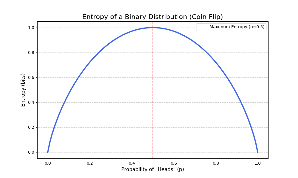
This plot clearly shows that our uncertainty about the coin flip’s outcome is highest when both outcomes are equally likely.
AI/ML Application Examples
Now, let’s see how cross-entropy is used in a real machine learning framework. We’ll use PyTorch to define a simple model and calculate the cross-entropy loss.
import torch
import torch.nn as nn

# --- Setup ---
# PyTorch's CrossEntropyLoss combines LogSoftmax and NLLLoss for numerical stability.
# It expects raw model outputs (logits), not probabilities from softmax.
loss_function = nn.CrossEntropyLoss()

# --- Example Data ---
# Batch size of 2, 4 classes
# Raw model outputs (logits) for two samples
logits = torch.tensor([
    [2.0, -1.0, 0.5, 0.1],  # Sample 1: Model strongly prefers class 0
    [-0.5, 1.5, 2.5, -1.0]   # Sample 2: Model strongly prefers class 2
], dtype=torch.float32)

# Ground truth labels (class indices)
# Sample 1 is class 0, Sample 2 is class 2.
labels = torch.tensor([0, 2], dtype=torch.long)

# --- Calculate Loss ---
loss = loss_function(logits, labels)

print(f"PyTorch CrossEntropyLoss: {loss.item():.4f}")

# --- Manual Verification (to build understanding) ---
# 1. Apply Softmax to get probabilities (Q)
softmax = nn.Softmax(dim=1)
probs = softmax(logits)
print("\nModel Probabilities (Q):")
print(probs)

# 2. Get the probability of the correct class for each sample
prob_correct_class_s1 = probs[0, 0] # Sample 1, correct class 0
prob_correct_class_s2 = probs[1, 2] # Sample 2, correct class 2

# 3. Calculate negative log-likelihood for each
nll_s1 = -torch.log(prob_correct_class_s1)
nll_s2 = -torch.log(prob_correct_class_s2)
print(f"\nNLL for Sample 1: {nll_s1.item():.4f}")
print(f"NLL for Sample 2: {nll_s2.item():.4f}")

# 4. Average the NLLs to get the final loss
manual_loss = (nll_s1 + nll_s2) / 2
print(f"\nManually Calculated Average Loss: {manual_loss.item():.4f}")
print(f"Matches PyTorch's output? {torch.isclose(loss, manual_loss)}")
Output:
PyTorch CrossEntropyLoss: 0.3612

Model Probabilities (Q):
tensor([[0.7030, 0.0350, 0.1569, 0.1051],
        [0.0344, 0.2541, 0.6907, 0.0209]])

NLL for Sample 1: 0.3524
NLL for Sample 2: 0.3701

Manually Calculated Average Loss: 0.3612
Matches PyTorch's output? True
This example demonstrates the end-to-end process within a leading AI framework. It shows that the CrossEntropyLoss function is a practical, efficient, and numerically stable implementation of the theoretical concept we’ve been studying.
Industry Applications and Case Studies
Information theory concepts are not confined to the research lab; they drive value in countless commercial applications.
- E-commerce and Recommendation Systems: Companies like Amazon and Netflix build models to predict which products a user will buy or which movies they will watch. These are fundamentally classification problems. The models are trained using cross-entropy loss to minimize the difference between their predicted probabilities and the actual user behavior. A lower cross-entropy loss translates directly to more accurate recommendations, leading to increased user engagement and sales. The business impact is measured in conversion rates, click-through rates, and ultimately, revenue.
- Natural Language Processing (NLP) and Machine Translation: Services like Google Translate or large language models like GPT-4 are trained on massive text datasets. At their core, these models predict the next word in a sequence. This is a classification problem over a vast vocabulary. The loss function is cross-entropy, measuring how well the model’s predicted probability distribution for the next word matches the actual next word in the training text. The performance of these models, and thus their business value in applications from chatbots to content creation, is directly tied to minimizing this loss.
- Medical Imaging and Diagnosis: In healthcare, AI models are trained to classify medical images (e.g., X-rays, MRIs) to detect diseases. A model might output probabilities for “healthy,” “benign tumor,” or “malignant tumor.” The true distribution is the radiologist’s diagnosis (a one-hot vector). Training with cross-entropy loss pushes the model to make its predictions align with expert medical opinion. The ROI is immense, measured in faster and more accurate diagnoses, reduced healthcare costs, and improved patient outcomes.
- A/B Testing Analysis in Web Development: A company might test two versions of a website (A and B) to see which one leads to more user sign-ups. User behavior on each version can be modeled as a probability distribution (e.g., P(sign-up), P(no sign-up)). KL divergence can be used to measure how much the behavior distribution for group B diverges from group A. A statistically significant KL divergence indicates that the change in the website had a real impact on user behavior, providing a rigorous, information-theoretic basis for making business decisions.
Best Practices and Common Pitfalls
While powerful, information-theoretic measures must be used correctly to be effective. Adhering to best practices and being aware of common pitfalls is crucial for any AI engineer.
- Embrace Numerical Stability: A common mistake is to implement cross-entropy by manually applying a softmax function and then a negative log-likelihood. This can be numerically unstable. For example, if the model is very confident and assigns a probability of 1.0 to the correct class, the softmax output might be slightly less than 1 due to floating-point inaccuracies, but if it outputs a value that rounds to 0 for an incorrect class, taking
log(0)will result in-inf. Modern deep learning frameworks provide combined functions (e.g.,torch.nn.CrossEntropyLoss,tf.keras.losses.CategoricalCrossentropy) that take raw logits as input. These functions use mathematical tricks like the log-sum-exp trick to provide stable, accurate gradients and should always be preferred. - Understand KL Divergence Asymmetry: A frequent point of confusion is treating KL divergence as a true distance. Remember, \(D_{KL}(P || Q) \neq D_{KL}(Q || P)\). The choice of which distribution is \(P\) and which is \(Q\) matters. For example, in \(D_{KL}(P || Q)\), the divergence is high if there is an event where \(P(x) > 0\) but \(Q(x) \to 0\) (Q incorrectly assigns zero probability to a possible event). In contrast, \(D_{KL}(Q || P)\) would be high if \(Q(x) > 0\) but \(P(x) \to 0\) (Q assigns probability to an impossible event). The choice depends on the application’s goal (e.g., avoiding false negatives vs. avoiding false positives).
- Match Loss Function to Model Output: Ensure the loss function matches the structure of your problem and your model’s final activation layer. Use binary cross-entropy for binary classification (with a sigmoid output), categorical cross-entropy for single-label multi-class classification (with a softmax output), and a different approach (like binary cross-entropy per class) for multi-label classification.
- Interpret Loss Values Correctly: The absolute value of the cross-entropy loss is not always interpretable on its own. A “high” loss could be due to a difficult problem (high inherent entropy) or a poor model. Focus on the trend of the loss during training. Is it decreasing steadily? Does the validation loss start to increase (a sign of overfitting)? Use it as a relative metric for model improvement and comparison.
- Beware of Label Smoothing: For classification, the “true” distribution is often a one-hot vector, which encourages the model to become overconfident, outputting probabilities very close to 1. This can hurt generalization. A technique called label smoothing modifies the target one-hot vector slightly, for example, changing \([0, 1, 0]\) to \([0.05, 0.9, 0.05]\). This discourages overconfidence and can act as a regularizer, often leading to better model performance.
Hands-on Exercises
These exercises are designed to reinforce the concepts learned in this chapter, progressing from basic calculations to practical application.
- Exercise 1: Manual Entropy Calculation
- Objective: Calculate and compare the entropy of two different probability distributions.
- Task: Consider two 6-sided dice. Die A is fair: \(P_A = [1/6, 1/6, 1/6, 1/6, 1/6, 1/6]\). Die B is loaded: \(P_B = [1/2, 1/4, 1/8, 1/16, 1/16, 0]\).
- Steps:
- Manually calculate the Shannon entropy \(H(P_A)\) in bits.
- Manually calculate the Shannon entropy \(H(P_B)\) in bits.
- Write a Python script using your
entropyfunction from earlier to verify your manual calculations.
- Expected Outcome: You should find that \(H(P_A) > H(P_B)\), confirming that the fair die has higher uncertainty.
- Exercise 2: Cross-Entropy for Model Evaluation
- Objective: Use cross-entropy to compare the performance of two simple models.
- Task: A 3-class classification problem has the true label
class 1(i.e., \(P = [0, 1, 0]\)).- Model 1 predicts the probability distribution \(Q_1 = [0.2, 0.6, 0.2]\).
- Model 2 predicts the probability distribution \(Q_2 = [0.3, 0.4, 0.3]\).
- Steps:
- Calculate the cross-entropy loss for Model 1.
- Calculate the cross-entropy loss for Model 2.
- Which model is better according to this loss function? Explain why.
- Expected Outcome: Model 1 should have a lower cross-entropy loss because it assigns a higher probability to the correct class.
- Exercise 3: Exploring KL Divergence Asymmetry
- Objective: Demonstrate that KL divergence is not a symmetric metric.
- Task: Consider two simple probability distributions over three events: \(P = [0.1, 0.8, 0.1]\) and \(Q = [0.5, 0.4, 0.1]\).
- Steps:
- Using your Python
kl_divergencefunction, calculate \(D_{KL}(P || Q)\). - Now, calculate \(D_{KL}(Q || P)\).
- Using your Python
- Expected Outcome: You will find that \(D_{KL}(P || Q) \neq D_{KL}(Q || P)\), providing a concrete example of the asymmetry of KL divergence.
Tools and Technologies
To work with information-theoretic concepts in AI, a few key libraries are essential.
- NumPy: The fundamental package for scientific computing in Python. It provides the N-dimensional array objects used to represent probability distributions and the mathematical functions (like
log,sum) needed for implementation. (e.g.,numpy==1.26.0) - SciPy: Built on NumPy, SciPy provides more advanced scientific tools.
scipy.stats.entropyis a pre-built, optimized function for calculating Shannon entropy and KL divergence, which is often more convenient than a manual implementation. (e.g.,scipy==1.13.0) - PyTorch: A leading deep learning framework. Its
torch.nn.CrossEntropyLossandtorch.nn.KLDivLossare the standard, numerically stable tools for using these concepts as loss functions in neural networks. (e.g.,torch==2.3.0) - TensorFlow/Keras: Another major deep learning framework. Its
tf.keras.losses.CategoricalCrossentropyandtf.keras.losses.KLDivergenceserve the same purpose as their PyTorch counterparts. (e.g.,tensorflow==2.16.1) - Matplotlib/Seaborn: These are the primary libraries for data visualization in Python. They are invaluable for plotting distributions, loss curves, and other diagnostics to build intuition and analyze model behavior.
Tip: When starting a new project, create a virtual environment and install these libraries using a
requirements.txtfile to ensure your development environment is reproducible.
Summary
This chapter provided a deep dive into the foundational information-theoretic concepts that are critical for modern AI engineering.
- Key Concepts: We defined information content (surprisal) as a measure of surprise, Shannon entropy as the average uncertainty of a distribution, cross-entropy as the cost of encoding one distribution with another, and KL divergence as the “distance” or information loss between two distributions.
- Core Relationship: We established the fundamental relationship: \(\text{Cross-Entropy} = \text{Entropy} + \text{KL Divergence}\). This explains why minimizing cross-entropy loss is equivalent to minimizing the KL divergence between the model’s predictions and the true data distribution.
- Practical Skills: You have learned to implement these metrics in Python and use them within major deep learning frameworks like PyTorch to build and train classification models.
- Real-World Applicability: These concepts are not merely theoretical; they are the engine behind state-of-the-art recommendation systems, machine translation services, and medical diagnostic tools. Understanding them is essential for any practicing AI engineer.
Further Reading and Resources
- Shannon, C. E. (1948). A Mathematical Theory of Communication. Bell System Technical Journal, 27(3), 379-423. The seminal paper that started the field. A must-read for historical context.
- Cover, T. M., & Thomas, J. A. (2006). Elements of Information Theory. Wiley-Interscience. The definitive textbook on information theory.
- Goodfellow, I., Bengio, Y., & Courville, A. (2016). Deep Learning. MIT Press. Chapter 3 provides an excellent overview of probability and information theory specifically for machine learning practitioners.
- PyTorch Documentation:
nn.CrossEntropyLoss. The official documentation provides technical details and usage examples for the most common loss function. - “Visual Information Theory” by Christopher Olah. An excellent blog post on distill.pub that uses beautiful visualizations to explain the core concepts of information theory. https://colah.github.io/posts/2015-09-Visual-Information/
- “A Gentle Introduction to Cross-Entropy for Machine Learning” by Jason Brownlee. A practical, code-focused tutorial on the Machine Learning Mastery blog. https://machinelearningmastery.com/cross-entropy-for-machine-learning/
Glossary of Terms
- Entropy (Shannon Entropy): A measure of the uncertainty, randomness, or average information content of a random variable. Denoted \(H(X)\).
- Cross-Entropy: A measure of the average number of bits needed to identify an event drawn from a true distribution \(P\), when the coding scheme is optimized for an estimated distribution \(Q\). It is widely used as a loss function in classification. Denoted \(H(P, Q)\).
- Kullback-Leibler (KL) Divergence: A measure of how one probability distribution \(P\) diverges from a second, expected probability distribution \(Q\). It quantifies the information lost when \(Q\) is used to approximate \(P\). Denoted \(D_{KL}(P || Q)\).
- Information Content (Surprisal): The amount of information gained from observing a single event, which is inversely proportional to its probability.
- Loss Function: A function that quantifies the “cost” or “error” of a model’s predictions compared to the ground truth. The goal of training is to minimize this function.
- One-Hot Encoding: A method of representing categorical data as binary vectors, where a single bit is “hot” (set to 1) to indicate the presence of a specific category.
- Softmax Function: An activation function that converts a vector of real numbers (logits) into a probability distribution, where each element is between 0 and 1 and the sum of all elements is 1.
