
Chapter 12: Multivariable Calculus and Gradient Descent
Chapter Objectives
Upon completing this chapter, students will be able to:
- Understand and compute partial derivatives and gradients for multivariable functions, forming the mathematical basis for optimization in higher dimensions.
- Analyze the topology of multidimensional optimization landscapes, identifying critical points such as local minima, maxima, and saddle points.
- Implement the Gradient Descent algorithm and its variants (Stochastic, Mini-Batch) from scratch in Python to solve optimization problems like linear regression.
- Design and visualize optimization paths using Python libraries like Matplotlib and NumPy to gain an intuitive understanding of how learning algorithms navigate parameter space.
- Optimize machine learning model training by selecting appropriate learning rates and applying advanced optimization algorithms like Adam and RMSprop.
- Deploy foundational calculus concepts to solve real-world AI problems, connecting theoretical mathematics to the practical training of machine learning models.
Introduction
Welcome to the engine room of modern machine learning. While previous chapters established the foundational building blocks of AI, this chapter introduces the core mathematical machinery that drives the learning process itself: multivariable calculus. In the world of AI, “learning” is synonymous with “optimization.” Whether we are training a neural network to recognize images, a language model to generate text, or a recommendation system to predict user preferences, the underlying task is to find the optimal set of parameters (or weights) for a model that minimizes its error on a given task. This error is quantified by a loss function, which is almost always a function of many, sometimes billions, of variables.
The central challenge, then, is to navigate a high-dimensional “landscape” defined by this loss function and find its lowest point. This is where multivariable calculus becomes indispensable. Concepts that might seem abstract, such as partial derivatives and gradients, are the very tools we use to determine the direction of “steepest descent” in this landscape, guiding our model’s parameters toward their optimal values. The primary algorithm that leverages these concepts is Gradient Descent, a simple yet profoundly powerful iterative method that forms the backbone of training for most deep learning models today.
In this chapter, we will bridge the gap between theoretical calculus and practical AI engineering. We will move from single-variable functions to the vast, high-dimensional spaces where modern AI models live. You will learn not just to compute gradients but to develop a deep intuition for what they represent. We will implement Gradient Descent from first principles, visualize its behavior, and explore the advanced, industry-standard optimizers like Adam that have made training today’s massive models feasible. By the end of this chapter, you will possess a fundamental understanding of how AI models learn and the mathematical engine that powers their optimization.
Technical Background
The transition from single-variable calculus to multivariable calculus is more than a simple extension; it is a leap into the conceptual framework required for nearly all modern machine learning. A simple model might have a few parameters, while a large language model like GPT-3 has 175 billion. Each parameter is a dimension in our optimization problem. To find the best version of the model, we must adjust all these parameters simultaneously to minimize a loss function. This section lays the groundwork for understanding how we can intelligently navigate this unimaginably complex, high-dimensional space.
From Single to Multiple Variables: The Leap into Higher Dimensions
In single-variable calculus, the derivative \(\frac{df}{dx}\) tells us the instantaneous rate of change of a function \(f(x)\) with respect to its single input variable \(x\). It represents the slope of the line tangent to the function’s curve at a given point. This single value tells us everything we need to know about how the function’s output changes as we make an infinitesimal change to its input.
Now, consider a function of two variables, \(f(x, y)\). How does its output change when we alter its inputs? The answer is more complex because we can move in infinitely many directions from any point \((x, y)\) in the input plane. We could change \(x\) while holding \(y\) constant, change \(y\) while holding \(x\) constant, or change both simultaneously. This requires a new tool: the partial derivative.,
Conceptual Leap: Single to Multivariable Calculus
| Concept | Single-Variable Calculus | Multivariable Calculus (for AI) |
|---|---|---|
| Function | f(x) |
L(θ₁, θ₂, ..., θₙ) (Loss Function) |
| Input | A single number, x. |
A vector of parameters, θ. |
| Geometric Shape | A 2D curve. | A high-dimensional surface (landscape). |
| Measure of Change | The Derivative, df/dx. A scalar value. |
The Gradient, ∇L(θ). A vector of partial derivatives. |
| Interpretation | The slope of the tangent line at a point. | The vector pointing in the direction of steepest ascent. |
| Optimization Goal | Find points where df/dx = 0. |
Find points where ∇L(θ) = 0 (minima, maxima, or saddle points). |
Partial Derivatives: Isolating Change in a Multidimensional World
A partial derivative measures the rate of change of a multivariable function with respect to one variable, while holding all other variables constant. It allows us to isolate the impact of a single input variable on the function’s output. For a function \(f(x, y)\), the partial derivative with respect to \(x\) is denoted \(\frac{\partial f}{\partial x}\) or \(f_x\). To compute it, we treat \(y\) as a constant and differentiate with respect to \(x\) using the standard rules of single-variable calculus.
For example, consider the function \(f(x, y) = 3x^2y + y^3\). To find \(\frac{\partial f}{\partial x}\), we treat \(y\) as a constant: \[ \frac{\partial f}{\partial x} = \frac{\partial}{\partial x}(3x^2y + y^3) = 6xy + 0 = 6xy \] To find \(\frac{\partial f}{\partial y}\), we treat \(x\) as a constant: \[ \frac{\partial f}{\partial y} = \frac{\partial}{\partial y}(3x^2y + y^3) = 3x^2 + 3y^2 \] Each partial derivative gives us the slope of the tangent line to the surface \(z = f(x, y)\) in the direction of one of the coordinate axes. \(\frac{\partial f}{\partial x}\) is the slope in the x-direction, and \(\frac{\partial f}{\partial y}\) is the slope in the y-direction. While useful, these two values alone do not capture the full picture of how the function changes in all directions. For that, we need to combine them into a single, powerful entity: the gradient.
The Gradient Vector: The Direction of Steepest Ascent
The gradient of a multivariable function is a vector that packages all the partial derivative information into a single object. For a function \(f(x_1, x_2, \ldots, x_n)\), its gradient, denoted \(\nabla f\) (pronounced “del f”), is a vector whose components are the partial derivatives of the function with respect to each variable: \[ \nabla f(x_1, \ldots, x_n) = \begin{bmatrix} \frac{\partial f}{\partial x_1} \ \frac{\partial f}{\partial x_2} \ \vdots \ \frac{\partial f}{\partial x_n} \end{bmatrix} \] The gradient vector has two profound properties that make it the cornerstone of optimization. First, at any given point in the function’s domain, the gradient vector points in the direction of the steepest ascent. That is, if you want to increase the function’s value as quickly as possible, you should move in the direction of the gradient. Second, the magnitude of the gradient vector, \(|\nabla f|\), represents the rate of change in that steepest direction. A large magnitude means the function is changing rapidly (a steep slope), while a small magnitude indicates a flatter region.
In machine learning, our goal is not to ascend but to descend the loss landscape to find a minimum. Therefore, the most important direction for us is the direction opposite to the gradient, \(-\nabla f\). This vector points in the direction of the steepest descent. This single insight is the entire foundation of the Gradient Descent algorithm. By repeatedly taking small steps in the direction of the negative gradient, we can iteratively walk “downhill” on the loss surface until we reach a valley, or a minimum.
Understanding the Optimization Landscape
The concept of a “landscape” is a powerful metaphor for visualizing the behavior of a loss function. For a model with two parameters, \(\theta_1\) and \(\theta_2\), the loss function \(L(\theta_1, \theta_2)\) can be plotted as a 3D surface, where the height \(z\) at any point \((\theta_1, \theta_2)\) represents the loss. Our goal is to find the coordinates \((\theta_1, \theta_2)\) that correspond to the lowest point on this surface. In reality, our landscapes have thousands or millions of dimensions, making direct visualization impossible. However, the mathematical principles remain the same, and the 2D/3D intuition is invaluable.
Visualizing Functions of Multiple Variables: Surfaces and Contours
A 3D surface plot is the most direct way to visualize a function of two variables. The input variables, say \(w_1\) and \(w_2\), form the x-y plane, and the function’s value, the loss \(L(w_1, w_2)\), is plotted on the z-axis. This creates a topographical map where hills represent high loss and valleys represent low loss.
Another powerful visualization tool is a contour plot. A contour plot is a 2D projection of the 3D surface, much like a topographical map of a mountain. Each contour line connects points of equal function value (equal loss). Where the contour lines are close together, the surface is steep. Where they are far apart, the surface is flat. The gradient at any point is always perpendicular to the contour line passing through that point, pointing “uphill” toward higher-value contours. The path of a Gradient Descent algorithm can be traced on this contour plot as a series of steps that cross the contour lines at right angles, moving from higher to lower contours.

Critical Points, Extrema, and Saddle Points
In our search for the minimum loss, we are interested in critical points: points where the gradient is the zero vector, \(\nabla f = \mathbf{0}\). At such points, the surface is “flat” in all axial directions. Critical points can be classified into three main types:
- Local Minima: These are the “valleys” in our landscape. At a local minimum, the function’s value is lower than at all nearby points. This is our target in optimization. A function can have multiple local minima, and the lowest of these is the global minimum.
- Local Maxima: These are the “peaks” of the landscape. The function’s value is higher than at all nearby points. In optimization, these are points to be avoided.
- Saddle Points: These are more complex and are extremely common in high-dimensional deep learning landscapes. A saddle point is a point that is a minimum along one direction but a maximum along another, like the shape of a horse’s saddle. From a saddle point, you can go downhill in some directions and uphill in others. Because the gradient is zero, a naive Gradient Descent algorithm can get stuck or slow down significantly near saddle points, posing a major challenge for optimization. Modern optimizers incorporate techniques like momentum to help “roll through” these tricky regions.
Understanding the existence of these different types of critical points is crucial. It explains why simply finding a point where \(\nabla L = \mathbf{0}\) is not sufficient. We need methods that are robust enough to escape saddle points and, ideally, find a “good” local minimum, even if the global minimum is computationally intractable to find.
The Core of Optimization: Gradient Descent
Gradient Descent is an iterative optimization algorithm for finding a local minimum of a differentiable function. It is the workhorse of modern machine learning, used to train everything from simple linear regression models to the most complex deep neural networks. Its power lies in its simplicity and effectiveness in high-dimensional spaces.
The Intuition: Descending the Mountain
Imagine you are standing on the side of a mountain in a thick fog, and your goal is to reach the lowest point in the valley. You can’t see the entire landscape, but you can feel the slope of the ground beneath your feet. The most straightforward strategy is to identify the direction of the steepest descent—the direction that goes “downhill” most sharply—and take a small step in that direction. You repeat this process: at your new location, you again find the steepest downhill direction and take another step. By repeating this simple action, you will trace a path down the mountainside, eventually arriving at a low point.
This is precisely the intuition behind Gradient Descent. The “mountain” is the loss function landscape. Your “position” is the current set of model parameters. The “slope of the ground” is the gradient of the loss function. The direction of “steepest descent” is the negative gradient, \(-\nabla L\). Each “step” is an update to the model’s parameters.
The Algorithm: Mathematical Formulation and Steps
Let’s formalize this intuition. Suppose we have a loss function \(L(\boldsymbol{\theta})\) that depends on a vector of parameters \(\boldsymbol{\theta}\). We want to find the \(\boldsymbol{\theta}\) that minimizes \(L\). The Gradient Descent algorithm proceeds as follows:
- Initialization: Start with an initial guess for the parameters, \(\boldsymbol{\theta}_0\). This can be a random set of values.
- Iteration: Repeat for a fixed number of epochs or until convergence: a. Compute the Gradient: Calculate the gradient of the loss function with respect to the current parameters, \(\nabla L(\boldsymbol{\theta}_t)\). This tells us the direction of steepest ascent. b. Update the Parameters: Adjust the parameters by taking a step in the opposite direction of the gradient. The size of the step is controlled by a hyperparameter called the learning rate, denoted by \(\alpha\). The update rule is: \[\boldsymbol{\theta}_{t+1} = \boldsymbol{\theta}_t – \alpha \nabla L(\boldsymbol{\theta}_t)\] This core equation is the heart of machine learning. It moves the parameters from their current state \(\boldsymbol{\theta}t\) to a new state \(\boldsymbol{\theta}{t+1}\) that is expected to have a lower loss.
- Termination: The process stops when a condition is met, such as the change in loss becoming very small, the magnitude of the gradient approaching zero, or a predefined number of iterations being reached.
graph TD
    subgraph "Gradient Descent Algorithm"
    A[Start] --> B{"Initialize Parameters<br><i>θ₀ (e.g., random)</i>"};
    style A fill:#283044,stroke:#283044,stroke-width:2px,color:#ebf5ee
    style B fill:#9b59b6,stroke:#9b59b6,stroke-width:1px,color:#ebf5ee

    B --> C[Start Iteration Loop];
    style C fill:#78a1bb,stroke:#78a1bb,stroke-width:1px,color:#283044

    C --> D("1- Compute Gradient<br><i>∇L(θₜ) = ∂L/∂θ</i><br>Finds direction of steepest ascent");
    style D fill:#e74c3c,stroke:#e74c3c,stroke-width:1px,color:#ebf5ee

    D --> E("2- Update Parameters<br><i>θₜ₊₁ = θₜ - α · ∇L(θₜ)</i><br>Take a step downhill");
    style E fill:#78a1bb,stroke:#78a1bb,stroke-width:1px,color:#283044

    E --> F{Convergence Check<br><i>e.g., max iterations reached? <br> or gradient magnitude ≈ 0?</i>};
    style F fill:#f39c12,stroke:#f39c12,stroke-width:1px,color:#283044

    F -- "No" --> C;
    F -- "Yes" --> G[End: Optimal Parameters Found<br><i>θ_final</i>];
    style G fill:#2d7a3d,stroke:#2d7a3d,stroke-width:2px,color:#ebf5ee
    end
The Learning Rate (α): A Critical Hyperparameter
The learning rate (\(\alpha\)) is arguably the most important hyperparameter in training machine learning models. It determines the size of the steps we take down the loss landscape. Choosing the right learning rate is critical:
- If \(\alpha\) is too small: The algorithm will take tiny steps, leading to very slow convergence. It might take an impractically long time to reach a minimum.
- If \(\alpha\) is too large: The algorithm might overshoot the minimum. Instead of descending into the valley, it could bounce from one side to the other, with the loss increasing rather than decreasing. In the worst case, the updates will diverge, leading to an explosion of parameter values.

Finding a good learning rate is often an empirical process, involving experimentation and techniques like learning rate schedules, where \(\alpha\) is decreased over time as the training progresses and the model gets closer to a minimum.
Tip: A common strategy is to start with a relatively high learning rate and gradually decrease it. This allows the model to make significant progress early on and then fine-tune its parameters as it approaches a solution.
Advanced Gradient-Based Optimization
While the basic (or “vanilla”) Gradient Descent algorithm is foundational, it has limitations, especially when applied to the complex, high-dimensional, and non-convex loss landscapes of deep neural networks. To address these challenges, several more sophisticated optimizers have been developed.
Stochastic and Mini-Batch Gradient Descent
In standard Gradient Descent (often called Batch Gradient Descent), computing the gradient \(\nabla L(\boldsymbol{\theta})\) requires evaluating the loss over the entire training dataset. For datasets with millions of examples, this is computationally prohibitive for each and every step. Two main variants solve this problem:
- Stochastic Gradient Descent (SGD): Instead of the whole dataset, SGD approximates the gradient by computing it for a single, randomly chosen training example at each step. This makes each update extremely fast. The path taken by SGD is much noisier and more erratic than Batch GD, but this randomness can be beneficial, helping it to escape shallow local minima and saddle points.
- Mini-Batch Gradient Descent: This is the most common approach used in practice. It strikes a balance between the stability of Batch GD and the speed of SGD. In this method, the gradient is computed on a small, random subset of the data called a “mini-batch” (e.g., 32, 64, or 256 examples). This provides a good estimate of the true gradient while being computationally efficient. It also offers a smoother convergence path than SGD.
Momentum and Adaptive Learning Rate Algorithms (Adam, RMSprop)
Even with mini-batches, optimization can be slow, especially in regions with high curvature or near saddle points. Advanced optimizers introduce concepts to accelerate convergence.
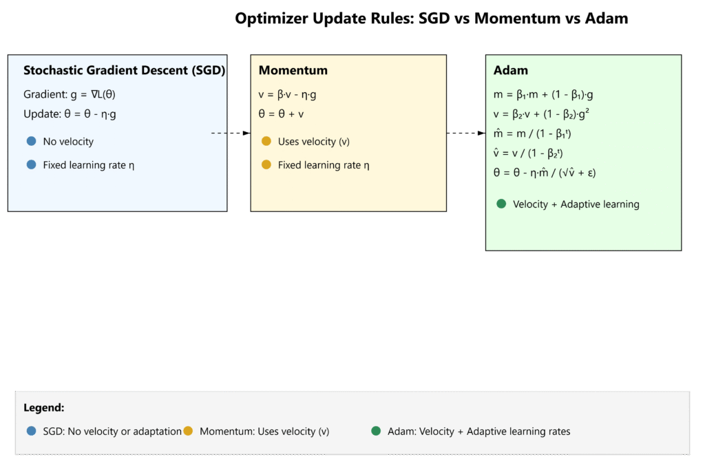
- Momentum: This method adds a “memory” of past updates to the current update. It introduces a velocity term that accumulates a fraction of the past gradients. The update rule can be thought of as a heavy ball rolling down the loss surface; it gathers momentum in consistent downhill directions and is less likely to be deflected by small bumps or get stuck in flat regions. The update becomes: \[ \mathbf{v}_{t+1} = \beta \mathbf{v}_t + (1-\beta) \nabla L(\boldsymbol{\theta}t) \] \[ \boldsymbol{\theta}{t+1} = \boldsymbol{\theta}t – \alpha \mathbf{v}{t+1} \] where \(\beta\) is the momentum coefficient, typically around 0.9.
- Adaptive Learning Rates (RMSprop, Adam): These algorithms go a step further by maintaining a per-parameter learning rate that adapts during training. The intuition is that some parameters may need larger updates while others require smaller, more fine-grained adjustments.
- RMSprop (Root Mean Square Propagation) divides the learning rate for a weight by a running average of the magnitudes of recent gradients for that weight.
- Adam (Adaptive Moment Estimation) is the de facto standard optimizer for most deep learning applications today. It combines the ideas of both momentum and adaptive learning rates. It maintains two moving averages for each parameter: one for the first moment of the gradient (like momentum) and one for the second moment (the uncentered variance). This allows it to compute individual, adaptive learning rates for each parameter, making it robust, efficient, and often requiring less manual tuning of the learning rate.
Practical Examples and Implementation
Theory is best understood through practice. In this section, we will translate the mathematical concepts of gradients and optimization into working Python code. We will use standard scientific computing libraries to demonstrate how these foundational ideas are implemented and applied to solve a classic machine learning problem.
Mathematical Concept Implementation
Before building a full machine learning model, let’s see how to compute gradients programmatically. We can use SymPy for symbolic differentiation to find the exact analytical form of the gradient, and NumPy for the numerical computation.
Let’s consider the function \(f(w_1, w_2) = w_1^2 + 2w_2^2\). This is a simple paraboloid with a global minimum at \((0, 0)\).
import numpy as np
import sympy as sp
import matplotlib.pyplot as plt
from mpl_toolkits.mplot3d import Axes3D

# --- Symbolic Gradient Calculation with SymPy ---
print("--- Symbolic Gradient Calculation ---")
# Define symbols
w1_sym, w2_sym = sp.symbols('w1 w2')

# Define the function
f_sym = w1_sym**2 + 2*w2_sym**2

# Calculate partial derivatives
df_dw1 = sp.diff(f_sym, w1_sym)
df_dw2 = sp.diff(f_sym, w2_sym)

# The gradient vector
gradient_sym = [df_dw1, df_dw2]

print(f"Function f(w1, w2) = {f_sym}")
print(f"Partial derivative w.r.t w1: ∂f/∂w1 = {df_dw1}")
print(f"Partial derivative w.r.t w2: ∂f/∂w2 = {df_dw2}")
print(f"Gradient vector ∇f = {gradient_sym}\n")


# --- Numerical Gradient Calculation with NumPy ---
print("--- Numerical Gradient Calculation ---")
# Define the function and its gradient in a way NumPy can use
# We use the results from SymPy to create the gradient function
def f(w):
    """The function f(w1, w2) = w1^2 + 2*w2^2"""
    return w[0]**2 + 2*w[1]**2

def grad_f(w):
    """The gradient of f(w1, w2)"""
    return np.array([2*w[0], 4*w[1]])

# Calculate the gradient at a specific point, e.g., (w1, w2) = (3, 4)
point = np.array([3, 4])
gradient_at_point = grad_f(point)

print(f"The function value at {point} is: {f(point)}")
print(f"The gradient at {point} is: {gradient_at_point}")
print("This vector [6, 16] points in the direction of steepest ascent from (3, 4).")
This code first uses SymPy to perform symbolic differentiation, giving us the general formula for the gradient. Then, it implements these formulas in NumPy to calculate the specific gradient vector at an arbitrary point. This vector, \([6, 16]\), tells us that from the point \((3, 4)\), the function increases most rapidly in this direction. For Gradient Descent, we would move in the opposite direction, \([-6, -16]\).
--- Symbolic Gradient Calculation ---
Function f(w1, w2) = w1**2 + 2*w2**2
Partial derivative w.r.t w1: ∂f/∂w1 = 2*w1
Partial derivative w.r.t w2: ∂f/∂w2 = 4*w2
Gradient vector ∇f = [2*w1, 4*w2]

--- Numerical Gradient Calculation ---
The function value at [3 4] is: 41
The gradient at [3 4] is: [ 6 16]
This vector [6, 16] points in the direction of steepest ascent from (3, 4).
AI/ML Application Examples
Now, let’s apply Gradient Descent to a core machine learning task: linear regression. Our goal is to find the best-fit line \(y = mx + b\) for a set of data points. In our terminology, the parameters to optimize are \(\boldsymbol{\theta} = [m, b]\). The loss function is typically the Mean Squared Error (MSE):
\[ L(m, b) = \frac{1}{N} \sum_{i=1}^{N} (y_i – (mx_i + b))^2 \]
We need the partial derivatives of \(L\) with respect to \(m\) and \(b\): \[ \frac{\partial L}{\partial m} = \frac{2}{N} \sum_{i=1}^{N} -x_i(y_i – (mx_i + b)) \] \[ \frac{\partial L}{\partial b} = \frac{2}{N} \sum_{i=1}^{N} -(y_i – (mx_i + b)) \]
Let’s implement this from scratch.
# --- Gradient Descent for Linear Regression ---
print("\n--- Implementing Gradient Descent for Linear Regression ---")

# Generate some sample data
np.random.seed(42)
X = 2 * np.random.rand(100, 1)
y = 4 + 3 * X + np.random.randn(100, 1) # True line: y = 3x + 4

# Add a bias term (for b) to X, so X_b is [1, x_i] for each row
X_b = np.c_[np.ones((100, 1)), X]

# Hyperparameters
learning_rate = 0.1
n_iterations = 1000
m = 100 # Number of data points

# Initialize parameters (theta = [b, m]) randomly
theta = np.random.randn(2, 1)

print(f"Initial parameters (b, m): {theta.ravel()}")

# Store loss history for plotting
loss_history = []

# Gradient Descent loop
for iteration in range(n_iterations):
    # Predictions
    predictions = X_b.dot(theta)

    # Errors
    errors = predictions - y

    # Calculate gradients
    gradients = 2/m * X_b.T.dot(errors)

    # Update parameters
    theta = theta - learning_rate * gradients

    # Calculate and store loss
    loss = np.mean(errors**2)
    loss_history.append(loss)

print(f"Final parameters (b, m) after {n_iterations} iterations: {theta.ravel()}")
print("The true values were b=4, m=3. Our algorithm found a close approximation.")

# Plotting the result
plt.figure(figsize=(14, 6))

# Plot 1: The regression line
plt.subplot(1, 2, 1)
plt.scatter(X, y)
plt.plot(X, X_b.dot(theta), color='red', linewidth=3, label='Fitted Line')
plt.title('Linear Regression with Gradient Descent')
plt.xlabel('X')
plt.ylabel('y')
plt.legend()

# Plot 2: The loss curve
plt.subplot(1, 2, 2)
plt.plot(range(n_iterations), loss_history)
plt.title('Loss Curve (MSE)')
plt.xlabel('Iteration')
plt.ylabel('Loss')
plt.grid(True)

plt.tight_layout()
plt.show()

This example demonstrates the entire process: we define a model (linear equation), a loss function (MSE), calculate its gradients, and iteratively update the model’s parameters to minimize the loss. The resulting plots clearly show the algorithm finding a line that fits the data well and the loss decreasing steadily over time.
--- Symbolic Gradient Calculation ---
Function f(w1, w2) = w1**2 + 2*w2**2
Partial derivative w.r.t w1: ∂f/∂w1 = 2*w1
Partial derivative w.r.t w2: ∂f/∂w2 = 4*w2
Gradient vector ∇f = [2*w1, 4*w2]

--- Numerical Gradient Calculation ---
The function value at [3 4] is: 41
The gradient at [3 4] is: [ 6 16]
This vector [6, 16] points in the direction of steepest ascent from (3, 4).

--- Implementing Gradient Descent for Linear Regression ---
Initial parameters (b, m): [0.01300189 1.45353408]
Final parameters (b, m) after 1000 iterations: [4.21509616 2.77011339]
The true values were b=4, m=3. Our algorithm found a close approximation.
Visualization and Interactive Examples
Visualizing the path of Gradient Descent on a contour plot provides powerful intuition. Let’s plot the MSE loss landscape for our linear regression problem and trace the steps our algorithm took.
import numpy as np
import sympy as sp
import matplotlib.pyplot as plt
from mpl_toolkits.mplot3d import Axes3D

# --- Symbolic Gradient Calculation with SymPy ---
print("--- Symbolic Gradient Calculation ---")
# Define symbols
w1_sym, w2_sym = sp.symbols('w1 w2')

# Define the function
f_sym = w1_sym**2 + 2*w2_sym**2

# Calculate partial derivatives
df_dw1 = sp.diff(f_sym, w1_sym)
df_dw2 = sp.diff(f_sym, w2_sym)

# The gradient vector
gradient_sym = [df_dw1, df_dw2]

print(f"Function f(w1, w2) = {f_sym}")
print(f"Partial derivative w.r.t w1: ∂f/∂w1 = {df_dw1}")
print(f"Partial derivative w.r.t w2: ∂f/∂w2 = {df_dw2}")
print(f"Gradient vector ∇f = {gradient_sym}\n")


# --- Numerical Gradient Calculation with NumPy ---
print("--- Numerical Gradient Calculation ---")
# Define the function and its gradient in a way NumPy can use
# We use the results from SymPy to create the gradient function
def f(w):
    """The function f(w1, w2) = w1^2 + 2*w2^2"""
    return w[0]**2 + 2*w[1]**2

def grad_f(w):
    """The gradient of f(w1, w2)"""
    return np.array([2*w[0], 4*w[1]])

# Calculate the gradient at a specific point, e.g., (w1, w2) = (3, 4)
point = np.array([3, 4])
gradient_at_point = grad_f(point)

print(f"The function value at {point} is: {f(point)}")
print(f"The gradient at {point} is: {gradient_at_point}")
print("This vector [6, 16] points in the direction of steepest ascent from (3, 4).")

# --- Gradient Descent for Linear Regression ---
print("\n--- Implementing Gradient Descent for Linear Regression ---")

# Generate some sample data
np.random.seed(42)
X = 2 * np.random.rand(100, 1)
y = 4 + 3 * X + np.random.randn(100, 1) # True line: y = 3x + 4

# Add a bias term (for b) to X, so X_b is [1, x_i] for each row
X_b = np.c_[np.ones((100, 1)), X]

# Hyperparameters
learning_rate = 0.1
n_iterations = 1000
m = 100 # Number of data points

# Initialize parameters (theta = [b, m]) randomly
theta = np.random.randn(2, 1)

print(f"Initial parameters (b, m): {theta.ravel()}")

# Store loss history for plotting
loss_history = []

# Gradient Descent loop
for iteration in range(n_iterations):
    # Predictions
    predictions = X_b.dot(theta)

    # Errors
    errors = predictions - y

    # Calculate gradients
    gradients = 2/m * X_b.T.dot(errors)

    # Update parameters
    theta = theta - learning_rate * gradients

    # Calculate and store loss
    loss = np.mean(errors**2)
    loss_history.append(loss)

print(f"Final parameters (b, m) after {n_iterations} iterations: {theta.ravel()}")
print("The true values were b=4, m=3. Our algorithm found a close approximation.")

# --- Visualizing the Optimization Path ---
print("\n--- Visualizing the Optimization Path ---")

# Function to compute MSE loss for given theta
def compute_loss(theta, X_b, y):
    m = len(y)
    predictions = X_b.dot(theta)
    errors = predictions - y
    return np.mean(errors**2)

# Create a grid of theta values (b and m)
b_vals = np.linspace(0, 8, 100)
m_vals = np.linspace(0, 6, 100)
B, M = np.meshgrid(b_vals, m_vals)

# Compute loss for each point on the grid
losses = np.zeros((100, 100))
for i in range(100):
    for j in range(100):
        theta_ij = np.array([[B[i, j]], [M[i, j]]])
        losses[i, j] = compute_loss(theta_ij, X_b, y)

# Run Gradient Descent again to store the path
theta = np.random.randn(2, 1) # Re-initialize
theta_path = [theta]
learning_rate = 0.1
n_iterations = 50

for iteration in range(n_iterations):
    gradients = 2/m * X_b.T.dot(X_b.dot(theta) - y)
    theta = theta - learning_rate * gradients
    theta_path.append(theta)

theta_path = np.array(theta_path)

# Plotting the contour plot with the path
plt.figure(figsize=(8, 8))
plt.contour(B, M, losses, levels=np.logspace(0, 3, 20), cmap='viridis')
plt.plot(theta_path[:, 0], theta_path[:, 1], 'r-o', label='GD Path')
plt.plot(4, 3, 'g*', markersize=15, label='True Minimum (4, 3)') # True values
plt.title('Gradient Descent Path on Loss Contour Plot')
plt.xlabel('Intercept (b)')
plt.ylabel('Slope (m)')
plt.legend()
plt.axis('equal')
plt.grid(True)
plt.show()
This visualization is incredibly insightful. The concentric ellipses are the contour lines of the loss function. The red line shows the step-by-step path our algorithm takes, starting from a random point and moving progressively toward the center (the green star), which represents the minimum loss. Notice how each step is perpendicular to the contour line it crosses, visually confirming that the algorithm is moving in the direction of steepest descent.
Computational Exercises
To solidify your understanding, perform these exercises.
- Manual Gradient Calculation: For the function \(f(w_1, w_2) = (w_1 – 5)^2 + (w_2 + 2)^2\), manually calculate the gradient \(\nabla f\). Then, compute the gradient vector at the point \((w_1, w_2) = (7, -1)\). What is the first update step for Gradient Descent starting at this point with a learning rate \(\alpha = 0.1\)?
- Solution Hint: \(\frac{\partial f}{\partial w_1} = 2(w_1 – 5)\) and \(\frac{\partial f}{\partial w_2} = 2(w_2 + 2)\). The update rule is \(\boldsymbol{\theta}_{1} = \boldsymbol{\theta}_0 – \alpha \nabla f(\boldsymbol{\theta}_0)\).
- Code Implementation: Write a Python function
gradient_descentthat takes a gradient functiongrad_f, an initial pointw_init, a learning ratelr, and a number of iterationsn_iteras input. It should return the final point and a history of all points visited. Test it on the function from exercise 1.
import numpy as np
import sympy as sp
import matplotlib.pyplot as plt
from mpl_toolkits.mplot3d import Axes3D

# --- Symbolic Gradient Calculation with SymPy ---
print("--- Symbolic Gradient Calculation ---")
# Define symbols
w1_sym, w2_sym = sp.symbols('w1 w2')

# Define the function
f_sym = w1_sym**2 + 2*w2_sym**2

# Calculate partial derivatives
df_dw1 = sp.diff(f_sym, w1_sym)
df_dw2 = sp.diff(f_sym, w2_sym)

# The gradient vector
gradient_sym = [df_dw1, df_dw2]

print(f"Function f(w1, w2) = {f_sym}")
print(f"Partial derivative w.r.t w1: ∂f/∂w1 = {df_dw1}")
print(f"Partial derivative w.r.t w2: ∂f/∂w2 = {df_dw2}")
print(f"Gradient vector ∇f = {gradient_sym}\n")


# --- Numerical Gradient Calculation with NumPy ---
print("--- Numerical Gradient Calculation ---")
# Define the function and its gradient in a way NumPy can use
# We use the results from SymPy to create the gradient function
def f(w):
    """The function f(w1, w2) = w1^2 + 2*w2^2"""
    return w[0]**2 + 2*w[1]**2

def grad_f(w):
    """The gradient of f(w1, w2)"""
    return np.array([2*w[0], 4*w[1]])

# Calculate the gradient at a specific point, e.g., (w1, w2) = (3, 4)
point = np.array([3, 4])
gradient_at_point = grad_f(point)

print(f"The function value at {point} is: {f(point)}")
print(f"The gradient at {point} is: {gradient_at_point}")
print("This vector [6, 16] points in the direction of steepest ascent from (3, 4).")

# --- Gradient Descent for Linear Regression ---
print("\n--- Implementing Gradient Descent for Linear Regression ---")

# Generate some sample data
np.random.seed(42)
X = 2 * np.random.rand(100, 1)
y = 4 + 3 * X + np.random.randn(100, 1) # True line: y = 3x + 4

# Add a bias term (for b) to X, so X_b is [1, x_i] for each row
X_b = np.c_[np.ones((100, 1)), X]

# Hyperparameters
learning_rate = 0.1
n_iterations = 1000
m = 100 # Number of data points

# Initialize parameters (theta = [b, m]) randomly
theta = np.random.randn(2, 1)

print(f"Initial parameters (b, m): {theta.ravel()}")

# Store loss history for plotting
loss_history = []

# Gradient Descent loop
for iteration in range(n_iterations):
    # Predictions
    predictions = X_b.dot(theta)

    # Errors
    errors = predictions - y

    # Calculate gradients
    gradients = 2/m * X_b.T.dot(errors)

    # Update parameters
    theta = theta - learning_rate * gradients

    # Calculate and store loss
    loss = np.mean(errors**2)
    loss_history.append(loss)

print(f"Final parameters (b, m) after {n_iterations} iterations: {theta.ravel()}")
print("The true values were b=4, m=3. Our algorithm found a close approximation.")

# --- Visualizing the Optimization Path ---
print("\n--- Visualizing the Optimization Path ---")

# Function to compute MSE loss for given theta
def compute_loss(theta, X_b, y):
    m = len(y)
    predictions = X_b.dot(theta)
    errors = predictions - y
    return np.mean(errors**2)

# Create a grid of theta values (b and m)
b_vals = np.linspace(0, 8, 100)
m_vals = np.linspace(0, 6, 100)
B, M = np.meshgrid(b_vals, m_vals)

# Compute loss for each point on the grid
losses = np.zeros((100, 100))
for i in range(100):
    for j in range(100):
        theta_ij = np.array([[B[i, j]], [M[i, j]]])
        losses[i, j] = compute_loss(theta_ij, X_b, y)

# Run Gradient Descent again to store the path
theta = np.random.randn(2, 1) # Re-initialize
theta_path = [theta]
learning_rate = 0.1
n_iterations = 50

for iteration in range(n_iterations):
    gradients = 2/m * X_b.T.dot(X_b.dot(theta) - y)
    theta = theta - learning_rate * gradients
    theta_path.append(theta)

theta_path = np.array(theta_path)

# --- Solution to Computational Exercise 2 ---
def f_ex(w):
    return (w[0] - 5)**2 + (w[1] + 2)**2

def grad_f_ex(w):
    return np.array([2 * (w[0] - 5), 2 * (w[1] + 2)])

def gradient_descent(grad_f, w_init, lr, n_iter):
    w = w_init
    path = [w]
    for _ in range(n_iter):
        grad = grad_f(w)
        w = w - lr * grad
        path.append(w)
    return w, np.array(path)

# Test the function
initial_point = np.array([7.0, -1.0])
learning_rate = 0.1
iterations = 50

final_point, path = gradient_descent(grad_f_ex, initial_point, learning_rate, iterations)

print(f"\n--- Computational Exercise Result ---")
print(f"Starting point: {initial_point}")
print(f"Final point after {iterations} iterations: {final_point}")
print("The true minimum is at (5, -2).")
--- Computational Exercise Result ---
Starting point: [ 7. -1.]
Final point after 50 iterations: [ 5.00002854 -1.99998573]
The true minimum is at (5, -2).
Real-World Problem Applications
The principles of Gradient Descent extend directly to training complex deep neural networks. For a task like image classification using a neural network, the loss function (e.g., Cross-Entropy Loss) is a highly complex, non-convex function of millions of weight parameters. The process is conceptually identical:
- Input a mini-batch of images and their labels.
- Perform a forward pass: push the image data through the network to get predictions.
- Calculate the loss by comparing predictions to true labels.
- Perform a backward pass (backpropagation): this is a computationally efficient algorithm that uses the chain rule of calculus to calculate the gradient of the loss with respect to every single weight in the network.
- Use an optimizer (like Adam) to update all weights according to the update rule: \(\boldsymbol{\theta}_{t+1} = \boldsymbol{\theta}_t – \alpha \nabla L(\boldsymbol{\theta}_t)\).
Every time you hear that a model like ResNet or a Transformer is being “trained,” it is this fundamental process of iterative, gradient-based optimization that is taking place on a massive scale.
Industry Applications and Case Studies
The application of multivariable calculus and gradient-based optimization is not an academic exercise; it is the engine driving billions of dollars of value across countless industries. The ability to optimize high-dimensional functions is what transforms data into actionable intelligence.
- E-commerce and Media: Recommendation Systems (Netflix, Amazon)
- Application: Collaborative filtering models predict what a user might like based on their past behavior and the behavior of similar users. The model’s parameters represent latent features of users and items.
- Technical Implementation: The problem is framed as minimizing a loss function (e.g., RMSE) between predicted and actual user ratings. This loss function is a function of the latent feature vectors. Gradient Descent (often with advanced variants like Adam) is used to learn the optimal feature vectors for all users and items, a space that can have millions of dimensions.
- Business Impact: At Netflix, personalized recommendations are credited with saving over $1 billion per year by reducing customer churn. Effective recommendations drive engagement, increase sales, and improve customer satisfaction.
- Finance: Algorithmic Trading and Risk Assessment
- Application: Models are trained to predict stock price movements or assess the credit risk of a loan applicant. The model parameters are weights applied to various input features (e.g., historical price data, market indicators, applicant’s financial history).
- Technical Implementation: A loss function is defined to penalize incorrect predictions (e.g., predicting a stock will go up when it goes down). Gradient-based optimizers adjust the model’s weights to minimize this loss on historical data. Performance is critical, and optimizations are made for low-latency inference.
- Business Impact: Successful trading algorithms can generate significant profits. Accurate risk models reduce financial losses from defaults and allow for more competitive pricing of financial products.
- Autonomous Vehicles: Perception and Path Planning (Tesla, Waymo)
- Application: Deep neural networks are used for object detection (identifying pedestrians, cars, traffic signs) from camera and sensor data. The network’s weights are the parameters being optimized.
- Technical Implementation: The network is trained on millions of labeled images. The loss function measures the discrepancy between the network’s predicted bounding boxes and the ground-truth labels. Backpropagation and an Adam optimizer are used to tune the millions of weights in the network to minimize this loss.
- Business Impact: Reliable perception is a prerequisite for safe autonomous driving. The entire viability of the multi-trillion dollar autonomous vehicle market rests on the ability to effectively train these massive neural networks using gradient-based optimization.
Best Practices and Common Pitfalls
Implementing gradient-based optimization effectively requires more than just understanding the math; it involves a set of practical skills and an awareness of common challenges. Adhering to best practices can be the difference between a model that trains successfully and one that fails to converge.
- Feature Scaling: This is one of the most critical preprocessing steps. If input features have vastly different scales (e.g., one feature ranges from 0-1 and another from 0-1,000,000), the loss landscape can become a very elongated, narrow valley. In this scenario, Gradient Descent will oscillate back and forth, taking a long time to converge. Always scale your features before training. Common methods include Standardization (scaling to zero mean and unit variance) or Normalization (scaling to a [0, 1] range).
- Proper Parameter Initialization: How you initialize your weights matters. Initializing all weights to zero is a common mistake, as it leads to all neurons in a layer learning the same thing (symmetric weights). A standard practice is to initialize weights with small random numbers drawn from a distribution like Glorot/Xavier or He initialization, which helps maintain a healthy variance of activations and gradients through the network.
- Choosing the Right Optimizer: While SGD is a great learning tool, for most practical deep learning applications, you should start with an adaptive optimizer like Adam. It is generally robust, converges quickly, and requires less manual tuning of the learning rate. However, it’s still worth understanding SGD with momentum, as it sometimes generalizes better in certain research contexts.
- Learning Rate Tuning: The learning rate is a hyperparameter you will almost always need to tune. If your loss is exploding, your learning rate is too high. If your loss is decreasing very slowly, it might be too low. Use learning rate finders (which gradually increase the LR and plot the loss) to identify a good range, and consider using learning rate schedules (e.g., cosine annealing or step decay) that decrease the learning rate during training for more stable convergence.
- Monitoring the Gradient: A common and difficult-to-debug problem is the vanishing or exploding gradient problem, where gradients become infinitesimally small or astronomically large during backpropagation in deep networks. This halts learning. Using activation functions like ReLU, proper weight initialization, and batch normalization are standard techniques to mitigate this. Tools like TensorBoard allow you to monitor the distribution and magnitude of your gradients during training, which can be invaluable for diagnostics.
Warning: Never use a learning rate without first checking the scale of your data and gradients. A learning rate of 0.01 might be perfect for one problem but cause another to diverge instantly. There is no single “best” learning rate.
Hands-on Exercises
These exercises are designed to reinforce the chapter’s concepts, progressing from foundational understanding to practical application.
- Visualizing Different Learning Rates:
- Objective: Understand the impact of the learning rate on the convergence of Gradient Descent.
- Task: Modify the “Visualizing the Optimization Path” code from the practical examples section. Run the Gradient Descent algorithm on the linear regression problem with three different learning rates: a very small one (e.g., 0.001), a good one (e.g., 0.1), and a very large one (e.g., 0.9).
- Expected Outcome: Generate three contour plots, each showing the path taken by the algorithm. The small learning rate should show slow progress, the good one should converge efficiently, and the large one should show overshooting and divergence. Add annotations to your plots explaining what is happening in each case.
- Implementing Mini-Batch Gradient Descent:
- Objective: Implement the most common variant of Gradient Descent used in practice.
- Task: Write a Python function to perform linear regression using Mini-Batch Gradient Descent. You will need to modify the existing Batch Gradient Descent code to loop through the training data in small, shuffled batches within each epoch.
- Guidance:
- Start with the Batch GD code for linear regression.
- Inside the main loop (the epoch loop), add another loop that iterates over mini-batches of the data.
- Before each epoch, shuffle the training data to ensure the batches are random.
- Calculate the gradient and perform the parameter update based on each mini-batch, not the full dataset.
- Verification: Compare the final parameters and the shape of the loss curve to the Batch Gradient Descent implementation. The Mini-Batch loss curve should be noisier but should still trend downwards to a similar solution.
- Team Challenge: Investigating Saddle Points:
- Objective: Analyze the behavior of different optimizers on a function with a saddle point.
- Task (Team of 2-3):
- Research and define a simple function with a saddle point, for example, \(f(x, y) = x^2 – y^2\). The point \((0, 0)\) is a saddle point.
- Student A: Implement Gradient Descent (vanilla SGD) to try to optimize this function starting from a point near the saddle point (e.g., \((0.1, 0.1)\)). Visualize the optimization path on a contour plot.
- Student B: Implement Gradient Descent with Momentum. Run it on the same problem and visualize its path.
- Expected Outcome: Prepare a short report or presentation comparing the two paths. You should observe that vanilla SGD slows down dramatically or gets stuck at the saddle point, while the momentum-based optimizer is able to “roll through” it and continue descending.
Tools and Technologies
The concepts in this chapter are brought to life by a powerful ecosystem of Python libraries designed for scientific computing and machine learning.
- NumPy: The fundamental package for numerical computation in Python. It provides efficient N-dimensional array objects (
ndarray) and a vast library of mathematical functions to operate on them. It is the bedrock for all numerical calculations in this chapter, from creating data to performing vector and matrix operations in the Gradient Descent updates.Installation: pip install numpy
- Matplotlib: The most widely used library for creating static, animated, and interactive visualizations in Python. We used it extensively to create 2D scatter plots, line graphs (for loss curves), 3D surface plots, and 2D contour plots, which are essential for building an intuitive understanding of optimization landscapes.
Installation: pip install matplotlib
- SymPy: A Python library for symbolic mathematics. Unlike NumPy which works with numbers, SymPy works with mathematical symbols and expressions. We used it to calculate the analytical partial derivatives and gradients of functions, which is extremely useful for verifying hand-calculated gradients and for understanding the underlying mathematical forms.
Installation: pip install sympy
- Scikit-learn: A high-level, user-friendly machine learning library. While we implemented linear regression from scratch for learning purposes, in a real project, you would likely use Scikit-learn’s
SGDRegressororLinearRegressionmodels. It provides pre-built, optimized, and tested implementations of many algorithms. It’s an excellent tool for applying these concepts without reinventing the wheel.Installation: pip install scikit-learn
- TensorFlow / PyTorch: These are the two dominant deep learning frameworks. When you move beyond simple models to deep neural networks, you will not be writing the backpropagation algorithm by hand. These frameworks provide automatic differentiation (
autograd) engines that compute gradients for even the most complex models automatically. They also include a suite of pre-built, highly optimized optimizers like Adam, RMSprop, and SGD. Understanding the principles from this chapter is essential for using these powerful tools effectively.
Summary
This chapter established the critical link between multivariable calculus and the core process of training AI models. We journeyed from foundational theory to practical, hands-on implementation.
- Key Concepts: We defined partial derivatives as a way to measure change in one dimension at a time and combined them into the gradient vector (\(\nabla f\)), which points in the direction of steepest ascent in a high-dimensional space.
- Optimization Landscape: We learned to visualize loss functions as surfaces and contour plots, identifying key features like local minima, maxima, and the challenging saddle points.
- Gradient Descent: We built the Gradient Descent algorithm from the ground up, based on the simple principle of taking iterative steps in the direction of the negative gradient (\(-\nabla f\)). We saw the critical role of the learning rate (\(\alpha\)) in controlling convergence.
- Advanced Optimizers: We explored the limitations of vanilla Gradient Descent and introduced its more practical and powerful variants: Stochastic Gradient Descent (SGD), Mini-Batch Gradient Descent, and adaptive methods like Momentum and Adam, which are the industry standard.
- Practical Skills: You gained hands-on experience implementing Gradient Descent in Python to solve a real machine learning problem (linear regression) and visualizing the optimization process to build deep, practical intuition.
The concepts in this chapter are not just a prerequisite for deep learning; they are its very essence. Every major breakthrough in AI in the last decade has been powered by models trained using these fundamental principles of gradient-based optimization. As you move on to study neural networks, you will see these ideas applied repeatedly at a massive scale.
Further Reading and Resources
- “Deep Learning” by Ian Goodfellow, Yoshua Bengio, and Aaron Courville: Chapter 4 (“Numerical Computation”) and Chapter 8 (“Optimization for Training Deep Models”) are the definitive, comprehensive references on this topic.
- 3Blue1Brown – “Gradient descent, how neural networks learn” video series: An outstanding and highly intuitive visual explanation of gradients and the core concepts of learning. https://www.youtube.com/watch?v=IHZwWFHWa-w
- CS231n: Convolutional Neural Networks for Visual Recognition (Stanford Course Notes): The “Optimization” and “Backpropagation” notes provide excellent, practical explanations and visualizations. Available online for free. https://cs231n.github.io/
- “Calculus on Manifolds” by Michael Spivak: For those seeking a deeper, more rigorous mathematical treatment of the underlying calculus in high dimensions.
- “An overview of gradient descent optimization algorithms” by Sebastian Ruder (2016): An influential and highly-cited blog post/paper that clearly explains the evolution from SGD to Adam and other modern optimizers.
- The NumPy, Matplotlib, and Scikit-learn Official Documentation: These are invaluable resources for practical implementation details, examples, and API references.
Glossary of Terms
- Partial Derivative (\(\frac{\partial f}{\partial x}\)): The derivative of a multivariable function with respect to one variable, holding all other variables constant. It measures the slope of the function along one axis.
- Gradient (\(\nabla f\)): A vector containing all the partial derivatives of a function. It points in the direction of the function’s steepest ascent.
- Loss Function (or Cost Function): A function that measures the error or “cost” of a model’s predictions compared to the true labels. The goal of training is to minimize this function.
- Gradient Descent: An iterative optimization algorithm that finds a local minimum of a function by repeatedly taking steps in the direction opposite to the gradient.
- Learning Rate (\(\alpha\)): A hyperparameter that controls the step size in each iteration of Gradient Descent.
- Epoch: One complete pass through the entire training dataset.
- Batch Gradient Descent: The version of Gradient Descent that computes the gradient using the entire training dataset for each update.
- Stochastic Gradient Descent (SGD): A variant of Gradient Descent that updates parameters using the gradient computed from a single, randomly chosen training example.
- Mini-Batch Gradient Descent: The most common variant of Gradient Descent, which computes the gradient on a small, random subset (a mini-batch) of the training data.
- Saddle Point: A critical point in a function’s landscape that is a minimum along one axis but a maximum along another. The gradient is zero, but it is not a local extremum.
- Adam (Adaptive Moment Estimation): A sophisticated and widely used optimization algorithm that combines the ideas of momentum and adaptive per-parameter learning rates.
