Chapter 10: Eigenvalues, Eigenvectors, and Matrix Decomp. Applications

Chapter Objectives

Upon completing this chapter, you will be able to:

Understand the fundamental mathematical theory behind eigenvalues, eigenvectors, and their relationship to linear transformations.
Analyze the properties of a matrix using eigenvalue decomposition and understand its geometric interpretation.
Implement algorithms for eigenvalue decomposition and Principal Component Analysis (PCA) from both a conceptual and practical standpoint using Python.
Design dimensionality reduction strategies for complex datasets, selecting appropriate techniques based on data characteristics and application requirements.
Optimize machine learning models by applying PCA for feature extraction, noise reduction, and performance improvement.
Deploy AI systems that leverage these mathematical foundations for tasks in computer vision, natural language processing, and data visualization.

Introduction

In the vast landscape of artificial intelligence, the ability to find meaningful patterns within high-dimensional data is paramount. From the pixels of an image to the thousands of features in a financial model, raw data is often too complex, noisy, and redundant to be used effectively. This is where the elegant concepts of eigenvalues and eigenvectors become indispensable tools for the modern AI engineer. At their core, these mathematical constructs allow us to distill the essence of a dataset, identifying the directions of maximum variance and uncovering the underlying structure that is often obscured by the sheer volume of information. This process, known as eigenvalue decomposition, is the engine behind one of the most powerful techniques in machine learning: Principal Component Analysis (PCA).

This chapter delves into the heart of these concepts, bridging the gap between abstract linear algebra and tangible, real-world applications. We will explore how eigenvectors represent the intrinsic axes of a transformation, remaining stable in direction while being scaled by their corresponding eigenvalues. This seemingly simple idea has profound implications, enabling us to rotate our perspective on a dataset to a new coordinate system where the features are uncorrelated and ranked by importance. By mastering these principles, you will gain the ability to dramatically reduce the dimensionality of your data, which not only accelerates model training but also mitigates the “curse of dimensionality,” leading to more robust and generalizable AI systems. We will move from the theoretical foundations to practical implementation, equipping you with the skills to build, analyze, and deploy sophisticated machine learning pipelines that are both computationally efficient and highly effective.

Technical Background

The journey into advanced machine learning techniques is paved with the foundational principles of linear algebra. Among the most critical of these are the concepts of eigenvalues and eigenvectors, which provide a deep insight into the properties of matrices and the linear transformations they represent. Understanding them is not merely an academic exercise; it is essential for grasping the mechanics of dimensionality reduction, data compression, and the internal workings of many sophisticated algorithms that power modern AI.

Fundamental Concepts and Definitions

At its core, linear algebra is the study of vectors, vector spaces, and the linear transformations that map vectors from one space to another. These transformations, which include rotation, scaling, and shearing, can be represented by matrices. While a matrix can transform a vector in a multitude of ways, eigenvectors are special. They are the vectors that, when subjected to the transformation, do not change their direction. Their orientation remains invariant, and the transformation’s only effect is to scale them by a certain factor. This scaling factor is the eigenvalue.

Core Terminology and Mathematical Foundations

The formal definition encapsulates this relationship succinctly. For a given square matrix \(\mathbf{A}\) of size \(n \times n\), a non-zero vector \(\mathbf{v}\) is an eigenvector of \(\mathbf{A}\) if it satisfies the following equation:

\[\mathbf{A}\mathbf{v} = \lambda\mathbf{v}\]

Here, \(\mathbf{v}\) is the eigenvector, and \(\lambda\) is the corresponding eigenvalue, which is a scalar. This equation states that when the matrix \(\mathbf{A}\) acts upon the vector \(\mathbf{v}\), the result is a new vector that is simply the original vector \(\mathbf{v}\) scaled by the factor \(\lambda\). The direction of \(\mathbf{v}\) is preserved.

To find the eigenvalues and eigenvectors of a matrix \(\mathbf{A}\), we can rearrange the equation:

\[\mathbf{A}\mathbf{v} – \lambda\mathbf{v} = 0\]

We can introduce the identity matrix \(\mathbf{I}\) (an \(n \times n\) matrix with ones on the main diagonal and zeros elsewhere) to facilitate matrix subtraction:

\[\mathbf{A}\mathbf{v} – \lambda\mathbf{I}\mathbf{v} = 0\]

\[(\mathbf{A} – \lambda\mathbf{I})\mathbf{v} = 0\]

This equation reveals a crucial insight. We are looking for a non-zero vector \(\mathbf{v}\) that, when multiplied by the matrix \((\mathbf{A} – \lambda\mathbf{I})\), results in the zero vector. According to the principles of linear algebra, this is only possible if the matrix \((\mathbf{A} – \lambda\mathbf{I})\) is singular, meaning it does not have an inverse. A singular matrix is one whose determinant is zero. This gives us a way to solve for the eigenvalues:

\[\det(\mathbf{A} – \lambda\mathbf{I}) = 0\]

Solving this equation, known as the characteristic equation, yields a polynomial in \(\lambda\) of degree \(n\), called the characteristic polynomial. The roots of this polynomial are the eigenvalues of the matrix \(\mathbf{A}\). For an \(n \times n\) matrix, there will be \(n\) eigenvalues, although they may not all be distinct and can include complex numbers. Once an eigenvalue \(\lambda\) is found, it can be substituted back into the equation \((\mathbf{A} – \lambda\mathbf{I})\mathbf{v} = 0\) to solve for the corresponding eigenvector(s) \(\mathbf{v}\). Each eigenvalue has an associated eigenspace, which is the set of all eigenvectors corresponding to that eigenvalue, along with the zero vector.

The properties of eigenvalues and eigenvectors are deeply connected to the properties of the matrix itself. For instance, the sum of the eigenvalues of a matrix is equal to its trace (the sum of the elements on the main diagonal), and the product of the eigenvalues is equal to its determinant. For symmetric matrices (where \(\mathbf{A} = \mathbf{A}^\top\)), a class of matrices frequently encountered in machine learning (e.g., covariance matrices), the eigenvalues are always real numbers, and the eigenvectors corresponding to distinct eigenvalues are orthogonal. This orthogonality is a powerful property that we will exploit heavily in Principal Component Analysis.

Historical Development and Evolution

The concept of eigenvalues, though formalized in the 19th and 20th centuries, has roots that stretch back to the 18th century in the study of rotational motion and differential equations. Mathematicians like Leonhard Euler and Joseph-Louis Lagrange encountered these ideas when analyzing the principal axes of rotation of a rigid body. They discovered that there were certain axes around which the body’s angular velocity and angular momentum were parallel—a physical manifestation of the eigenvector-eigenvalue relationship.

However, it was Augustin-Louis Cauchy in the 1820s who first generalized these ideas and proved that symmetric matrices have real eigenvalues, a cornerstone result. The terms “eigenvalue” and “eigenvector” themselves are a hybrid of German and English. “Eigen” in German means “own,” “proper,” or “characteristic.” Thus, an eigenvector is a “characteristic vector” of a transformation. The term was first used in this context by David Hilbert in 1904, though the related concept of “characteristic roots” was already in use.

timeline
    title Evolution of Eigenvalue Concepts
    18th Century : Rotational Motion
         : Euler & Lagrange study principal axes of rotation.
         : Physical manifestation of eigenvector-eigenvalue relationship observed.
    1820s : Generalization
         : Cauchy proves symmetric matrices have real eigenvalues.
    1904 : Terminology
         : David Hilbert first uses the term "eigenvalue" (from German "eigen" meaning "own").
    Early 20th Century : Quantum Mechanics
         : Eigenvalues represent measurable quantities like energy and momentum.
         : Cemented the importance of eigenvalue problems in physics.
    Mid-20th Century : Computational Methods
         : Advent of digital computers spurs research.
         : Development of the QR algorithm for large matrices.
         : Unlocks applications in statistics and data analysis.

The development of quantum mechanics in the early 20th century provided a major impetus for the study of eigenvalues. In this domain, physical observables like energy, momentum, and spin are represented by operators (a generalization of matrices), and their eigenvalues represent the possible measurable values of those observables. The state of a system is described by a vector, which is an eigenvector of the observable operator. This profound connection cemented the importance of eigenvalue problems in modern physics and engineering. In the mid-20th century, with the advent of digital computing, numerical methods for calculating eigenvalues and eigenvectors for large matrices became a critical area of research, leading to the development of algorithms like the QR algorithm, which remains a standard today. This computational power unlocked the application of these concepts to statistics and, eventually, to machine learning, where they found a new and powerful role in data analysis.

The Power of Matrix Decomposition

Matrix decomposition, or factorization, is the process of breaking down a matrix into a product of simpler, constituent matrices. This is analogous to factoring an integer into its prime numbers. Such a decomposition can reveal deep properties of the matrix and make certain computations more efficient and stable. Eigenvalue decomposition, also known as spectral decomposition, is one of the most important forms of matrix decomposition.

Eigenvalue Decomposition (EVD)

For a square matrix \(\mathbf{A}\) that is diagonalizable, it can be decomposed into the following form:

\[\mathbf{A} = \mathbf{P}\mathbf{D}\mathbf{P}^{-1}\]

Where:

P is a square matrix whose columns are the eigenvectors of \(\mathbf{A}\).
D is a diagonal matrix whose diagonal entries are the corresponding eigenvalues of \(\mathbf{A}\).
P⁻¹ is the inverse of matrix \(\mathbf{P}\).

This decomposition is a restatement of the eigenvector equation \(\mathbf{A}\mathbf{v} = \lambda\mathbf{v}\) for all eigenvectors simultaneously. If we let the columns of \(\mathbf{P}\) be the eigenvectors \(\mathbf{v}_1, \mathbf{v}_2, \dots, \mathbf{v}_n\) and the diagonal elements of \(\mathbf{D}\) be the eigenvalues \(\lambda_1, \lambda_2, \dots, \lambda_n\), then the equation \(\mathbf{A}\mathbf{P} = \mathbf{P}\mathbf{D}\) holds. Multiplying by \(\mathbf{P}^{-1}\) on the right gives us the decomposition.

A particularly important case arises when \(\mathbf{A}\) is a real symmetric matrix. As mentioned earlier, its eigenvectors corresponding to distinct eigenvalues are orthogonal. If we normalize these eigenvectors (i.e., make them unit vectors), the matrix \(\mathbf{P}\) becomes an orthogonal matrix. An orthogonal matrix has the convenient property that its inverse is equal to its transpose (\(\mathbf{P}^{-1} = \mathbf{P}^\top\)). In this case, the eigenvalue decomposition simplifies to:

\[\mathbf{A} = \mathbf{P}\mathbf{D}\mathbf{P}^\top\]

This form is computationally much more stable and easier to work with, as calculating a transpose is trivial compared to calculating an inverse. Covariance matrices, which are central to PCA, are always symmetric, making this form of decomposition directly applicable.

The power of this decomposition lies in its ability to simplify matrix operations. For example, calculating the \(k\)-th power of \(\mathbf{A}\) becomes much easier:

\[\mathbf{A}^k = (\mathbf{P}\mathbf{D}\mathbf{P}^{-1})^k = \mathbf{P}\mathbf{D}^k\mathbf{P}^{-1}\]

Calculating \(\mathbf{D}^k\) is trivial, as it simply involves raising the diagonal elements (the eigenvalues) to the \(k\)-th power. This technique is used in applications ranging from calculating population growth models to rendering graphics in video games.

graph TD
    subgraph "Eigenvalue Decomposition (EVD)"
        A["`<b>Matrix A</b><br>(n x n Square Matrix)`"]
        style A fill:#e74c3c,stroke:#e74c3c,stroke-width:2px,color:#ebf5ee

        P["`<b>P</b><br>(Matrix of Eigenvectors)<br>[v₁, v₂, ..., vₙ]`"]
        style P fill:#78a1bb,stroke:#78a1bb,stroke-width:1px,color:#283044

        D["`<b>D</b><br>(Diagonal Matrix of Eigenvalues)<br>diag(λ₁, λ₂, ..., λₙ)`"]
        style D fill:#9b59b6,stroke:#9b59b6,stroke-width:1px,color:#ebf5ee

        P_inv["`<b>P⁻¹</b> or <b>Pᵀ</b><br>(Inverse or Transpose of P)`"]
        style P_inv fill:#78a1bb,stroke:#78a1bb,stroke-width:1px,color:#283044

        A --"Decomposes into"--> P
        A --"Decomposes into"--> D
        A --"Decomposes into"--> P_inv

        subgraph Reconstruction
            direction LR
            P_recon["`<b>P</b>`"]
            style P_recon fill:#78a1bb,stroke:#78a1bb,stroke-width:1px,color:#283044
            D_recon["`<b>D</b>`"]
            style D_recon fill:#9b59b6,stroke:#9b59b6,stroke-width:1px,color:#ebf5ee
            P_inv_recon["`<b>P⁻¹</b>`"]
            style P_inv_recon fill:#78a1bb,stroke:#78a1bb,stroke-width:1px,color:#283044
            A_recon["`<b>A</b><br>(Reconstructed)`"]
            style A_recon fill:#2d7a3d,stroke:#2d7a3d,stroke-width:2px,color:#ebf5ee

            P_recon --"Matrix Multiply"--> D_recon
            D_recon --"Matrix Multiply"--> P_inv_recon
            P_inv_recon --> A_recon
        end

        P --> P_recon
        D --> D_recon
        P_inv --> P_inv_recon
    end

    linkStyle 0 stroke-width:2px,fill:none,stroke:black;
    linkStyle 1 stroke-width:2px,fill:none,stroke:black;
    linkStyle 2 stroke-width:2px,fill:none,stroke:black;

Geometric Interpretation and Transformations

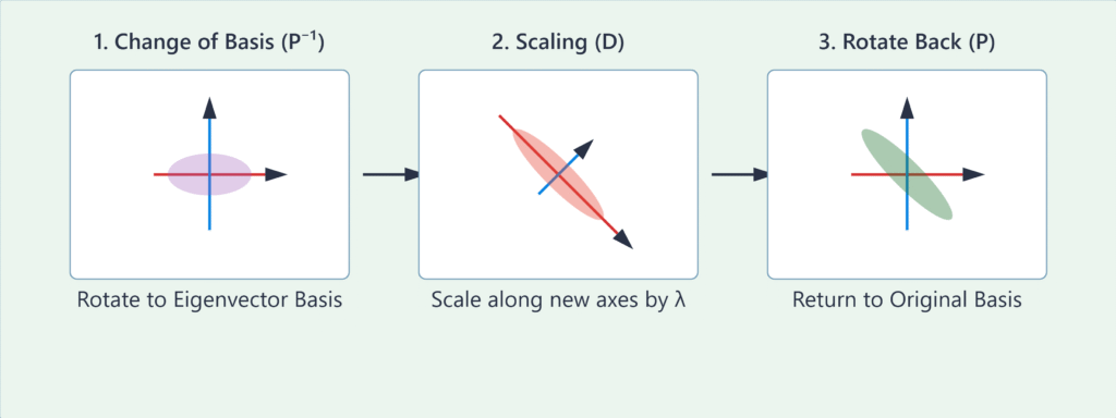
Eigenvalue decomposition provides a profound geometric interpretation of a linear transformation. Any linear transformation represented by a diagonalizable matrix \(\mathbf{A}\) can be thought of as a three-step process:

A change of basis (\(\mathbf{P}^{-1}\) or \(\mathbf{P}^\top\)): The transformation \(\mathbf{P}^{-1}\) rotates the coordinate system so that the new basis vectors are the eigenvectors of \(\mathbf{A}\). In this new basis, the transformation’s behavior becomes much simpler.
A scaling operation (\(\mathbf{D}\)): In the eigenvector basis, the transformation \(\mathbf{A}\) acts simply by stretching or compressing the space along the new axes. The scaling factor along each eigenvector axis is the corresponding eigenvalue \(\lambda\). If \(\lambda > 1\), it’s a stretch. If \(0 < \lambda < 1\), it’s a compression. If \(\lambda < 0\), it’s a reflection followed by a scaling.
A rotation back to the original basis (\(\mathbf{P}\)): The transformation \(\mathbf{P}\) rotates the coordinate system back to the original standard basis.

Therefore, eigenvalue decomposition reveals the “natural” axes of a transformation. It untangles the complex interplay of rotation, scaling, and shearing into a simple scaling operation along a special set of orthogonal axes. This is the key intuition behind PCA. When we apply this to a covariance matrix of a dataset, the eigenvectors point in the directions of maximum variance in the data, and the eigenvalues quantify how much variance exists along each of those directions.

Principal Component Analysis (PCA)

Principal Component Analysis is arguably the most widely used application of eigenvalue decomposition in machine learning. It is an unsupervised learning technique used for dimensionality reduction, data visualization, and feature extraction. The goal of PCA is to find a new set of orthogonal axes, called principal components, that are aligned with the directions of maximum variance in the data.

The PCA Algorithm

The process of performing PCA is a direct application of the concepts we’ve discussed. It can be summarized in the following steps:

Standardize the Data: PCA is sensitive to the scale of the features. If one feature has a much larger range than others, it will dominate the variance calculation. Therefore, the first step is to standardize the dataset so that each feature has a mean of 0 and a standard deviation of 1. For a data matrix \(\mathbf{X}\), where rows are samples and columns are features, we subtract the mean of each column from the column and then divide by its standard deviation.
Compute the Covariance Matrix: The next step is to understand how the different features in the dataset vary with respect to each other. This is captured by the covariance matrix. The covariance between two features measures their joint variability. A positive covariance indicates they tend to increase or decrease together, while a negative covariance indicates that one tends to increase as the other decreases. The covariance matrix \(\mathbf{C}\) for the standardized data is calculated as:[\mathbf{C} = \frac{1}{m-1} \mathbf{X}^\top\mathbf{X}]where \(m\) is the number of samples. The resulting matrix \(\mathbf{C}\) will be a square, symmetric matrix of size \(n \times n\), where \(n\) is the number of features. The diagonal elements of \(\mathbf{C}\) represent the variance of each feature, and the off-diagonal elements represent the covariance between pairs of features.
Perform Eigenvalue Decomposition on the Covariance Matrix: This is the core step of PCA. We compute the eigenvalues and eigenvectors of the covariance matrix \(\mathbf{C}\).[\mathbf{C} = \mathbf{P}\mathbf{D}\mathbf{P}^\top]The columns of \(\mathbf{P}\) are the eigenvectors, and the diagonal elements of \(\mathbf{D}\) are the eigenvalues. Because \(\mathbf{C}\) is symmetric, the eigenvectors (the columns of \(\mathbf{P}\)) will be orthogonal to each other. These eigenvectors are the principal components of the dataset. They represent the directions of maximum variance.
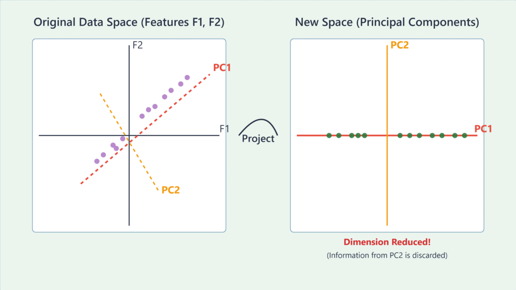
Sort Eigenvalues and Eigenvectors: The eigenvalues represent the magnitude of the variance along their corresponding eigenvector directions. We sort the eigenvalues in descending order. The eigenvector with the highest eigenvalue is the first principal component (PC1). It is the direction in which the data varies the most. The eigenvector with the second-highest eigenvalue is the second principal component (PC2), and so on. PC2 is orthogonal to PC1 and captures the next highest amount of variance.
Select Principal Components and Form the Projection Matrix: This is where dimensionality reduction happens. We decide how many principal components to keep. A common method is to look at the explained variance ratio, which is the fraction of the total variance that is captured by each principal component. The explained variance for the \(i\)-th component is \(\lambda_i / \sum_j \lambda_j\). We can choose to keep enough components to explain a certain percentage of the total variance, for example, 95%. If we decide to keep the top \(k\) components (where \(k < n\)), we form a projection matrix \(\mathbf{W}\) by taking the first \(k\) columns of the sorted eigenvector matrix \(\mathbf{P}\).
Project the Data onto the New Subspace: The final step is to transform the original standardized data \(\mathbf{X}\) into the new, lower-dimensional space. This is done by multiplying the data matrix \(\mathbf{X}\) by the projection matrix \(\mathbf{W}\):[\mathbf{X}_{\text{reduced}} = \mathbf{X}\mathbf{W}]

The resulting matrix \(\mathbf{X}_{\text{reduced}}\) will have dimensions \(m \times k\), where \(m\) is the number of samples and \(k\) is the new, reduced number of features. We have successfully reduced the dimensionality of our data from \(n\) to \(k\) while preserving the maximum possible variance.

flowchart TD
    A[Start: Original Dataset X] --> B{1- Standardize Data};
    style A fill:#283044,stroke:#283044,stroke-width:2px,color:#ebf5ee
    B --> C[2- Compute Covariance Matrix C];
    style B fill:#78a1bb,stroke:#78a1bb,stroke-width:1px,color:#283044
    C --> D[3- Perform Eigenvalue Decomposition on C];
    style C fill:#9b59b6,stroke:#9b59b6,stroke-width:1px,color:#ebf5ee
    D --> E{4- Sort Eigenvalues & Eigenvectors};
    style D fill:#e74c3c,stroke:#e74c3c,stroke-width:1px,color:#ebf5ee
    E --> F{5- Select k Principal Components};
    style E fill:#78a1bb,stroke:#78a1bb,stroke-width:1px,color:#283044
    F --> G[6- Form Projection Matrix W];
    style F fill:#f39c12,stroke:#f39c12,stroke-width:1px,color:#283044
    G --> H[7- Project Data: X_reduced = X_std * W];
    style G fill:#78a1bb,stroke:#78a1bb,stroke-width:1px,color:#283044
    H --> I[End: Lower-Dimensional Dataset];
    style H fill:#78a1bb,stroke:#78a1bb,stroke-width:1px,color:#283044
    style I fill:#2d7a3d,stroke:#2d7a3d,stroke-width:2px,color:#ebf5ee

    subgraph "Input/Output"
        A
        I
    end

    subgraph "Core PCA Steps"
        B
        C
        D
        E
        F
        G
        H
    end

Applications and Limitations

PCA is used across numerous domains. In computer vision, it’s used for facial recognition in a technique called “Eigenfaces,” where principal components of a large set of face images are used to create a feature space for identifying individuals. In finance, it’s used to analyze the risk of a portfolio of assets by identifying the principal components of asset returns. In natural language processing, it can be used to reduce the dimensionality of high-dimensional vector representations of words or documents.

However, PCA is not without its limitations. Its primary drawback is that the principal components, being linear combinations of the original features, can be difficult to interpret. While PC1 might capture the most variance, it may not be easily translatable back into a meaningful business or physical concept. Secondly, PCA assumes that the directions of maximum variance are the most important, which may not always be true, especially for classification tasks where the directions that best separate classes might have low variance. Finally, PCA is a linear technique. If the underlying structure of the data is highly non-linear, PCA may fail to find a meaningful low-dimensional representation. In such cases, non-linear dimensionality reduction techniques like t-SNE (t-Distributed Stochastic Neighbor Embedding) or autoencoders may be more appropriate.

graph TD
    subgraph Original Features
        direction LR
        F1(Feature 1)
        F2(Feature 2)
        F3(Feature 3)
        F4(Feature 4)
        F5(Feature 5)
    end
    style F1 fill:#9b59b6,stroke:#9b59b6,stroke-width:1px,color:#ebf5ee
    style F2 fill:#9b59b6,stroke:#9b59b6,stroke-width:1px,color:#ebf5ee
    style F3 fill:#9b59b6,stroke:#9b59b6,stroke-width:1px,color:#ebf5ee
    style F4 fill:#9b59b6,stroke:#9b59b6,stroke-width:1px,color:#ebf5ee
    style F5 fill:#9b59b6,stroke:#9b59b6,stroke-width:1px,color:#ebf5ee

    subgraph "Feature Selection"
        direction LR
        FS_Desc("Selects a subset of<br><i>original</i> features.")
        style FS_Desc fill:#ebf5ee,stroke:#78a1bb
        F1_sel(Feature 1)
        F3_sel(Feature 3)
        F5_sel(Feature 5)
    end
    style F1_sel fill:#2d7a3d,stroke:#2d7a3d,stroke-width:2px,color:#ebf5ee
    style F3_sel fill:#2d7a3d,stroke:#2d7a3d,stroke-width:2px,color:#ebf5ee
    style F5_sel fill:#2d7a3d,stroke:#2d7a3d,stroke-width:2px,color:#ebf5ee

    subgraph "PCA (Feature Extraction)"
        direction LR
        PCA_Desc("Creates <i>new</i> features<br>(Principal Components) from<br>linear combinations of originals.")
        style PCA_Desc fill:#ebf5ee,stroke:#78a1bb
        PC1("`PC1 = a*F1 + b*F2 + ...`")
        PC2("`PC2 = c*F1 + d*F2 + ...`")
    end
    style PC1 fill:#e74c3c,stroke:#e74c3c,stroke-width:1px,color:#ebf5ee
    style PC2 fill:#e74c3c,stroke:#e74c3c,stroke-width:1px,color:#ebf5ee

    F1 --> PCA_Desc
    F2 --> PCA_Desc
    F3 --> PCA_Desc
    F4 --> PCA_Desc
    F5 --> PCA_Desc

    F1 --> FS_Desc
    F3 --> FS_Desc
    F5 --> FS_Desc

    PCA_Desc --> PC1
    PCA_Desc --> PC2

    FS_Desc --> F1_sel
    FS_Desc --> F3_sel
    FS_Desc --> F5_sel

Practical Examples and Implementation

Theoretical understanding is the foundation, but true mastery comes from practical application. In this section, we will translate the mathematical concepts of eigenvalues, eigenvectors, and PCA into working Python code. We will use standard scientific computing libraries like NumPy for numerical operations, scikit-learn for high-level ML implementations, and Matplotlib/Seaborn for visualization.

Mathematical Concept Implementation

Let’s start by implementing eigenvalue decomposition from scratch using NumPy to solidify our understanding of the core mechanics.

Eigenvalue Decomposition with NumPy

NumPy provides a convenient function, numpy.linalg.eig(), which handles the complex calculations for us. Let’s define a simple 2×2 symmetric matrix and find its eigenvalues and eigenvectors.

Python

import numpy as np

# Define a symmetric matrix
A = np.array([[4, 2],
              [2, 7]])

print("Original Matrix A:\n", A)

# Calculate eigenvalues and eigenvectors
eigenvalues, eigenvectors = np.linalg.eig(A)

print("\nEigenvalues (λ):\n", eigenvalues)
print("\nEigenvectors (v) [as columns]:\n", eigenvectors)

# Verify the Av = λv relationship for the first eigenvector
lambda_1 = eigenvalues[0]
v_1 = eigenvectors[:, 0] # First column is the first eigenvector

# Calculate Av
Av1 = A @ v_1
# Calculate λv
lambda_v1 = lambda_1 * v_1

print("\nVerification for the first eigenpair:")
print("A * v1 =", Av1)
print("λ1 * v1 =", lambda_v1)

# Check if they are approximately equal
assert np.allclose(Av1, lambda_v1), "Verification failed!"
print("\nVerification successful: Av is indeed equal to λv.")

# Verify the decomposition A = PDPᵀ
# P is the matrix of eigenvectors
P = eigenvectors
# D is the diagonal matrix of eigenvalues
D = np.diag(eigenvalues)
# P transpose (since A is symmetric, P is orthogonal)
P_T = P.T

# Reconstruct A
A_reconstructed = P @ D @ P_T

print("\nReconstructed Matrix from PDPᵀ:\n", A_reconstructed)
assert np.allclose(A, A_reconstructed), "Decomposition failed!"
print("\nReconstruction successful.")

This code demonstrates the fundamental properties we discussed. It computes the eigenvalues and eigenvectors, verifies the core relationship \(\mathbf{A}\mathbf{v} = \lambda\mathbf{v}\), and confirms the spectral decomposition \(\mathbf{A} = \mathbf{P}\mathbf{D}\mathbf{P}^\top\). Running this code provides tangible proof of the theory.

AI/ML Application Examples

Now, let’s implement the full PCA algorithm. We will first do it step-by-step using NumPy to see the inner workings, and then show the much simpler implementation using scikit-learn.

PCA Implementation from Scratch

We will use the famous Iris dataset for this example. It has 4 features, and we will reduce it to 2 principal components for visualization.

Python

import numpy as np
import matplotlib.pyplot as plt
import seaborn as sns
from sklearn.datasets import load_iris

# 1. Load and prepare the data
iris = load_iris()
X = iris.data
y = iris.target
feature_names = iris.feature_names

print("Original data shape:", X.shape)

# 2. Standardize the data
X_std = (X - np.mean(X, axis=0)) / np.std(X, axis=0)

# 3. Compute the covariance matrix
cov_mat = np.cov(X_std, rowvar=False)
print("\nCovariance matrix shape:", cov_mat.shape)

# 4. Perform eigenvalue decomposition
eigenvalues, eigenvectors = np.linalg.eig(cov_mat)

# 5. Sort eigenvalues and eigenvectors
sorted_indices = np.argsort(eigenvalues)[::-1]
sorted_eigenvalues = eigenvalues[sorted_indices]
sorted_eigenvectors = eigenvectors[:, sorted_indices]

# 6. Select top k components (k=2)
k = 2
projection_matrix = sorted_eigenvectors[:, :k]
print("\nProjection matrix shape:", projection_matrix.shape)

# 7. Project the data
X_pca = X_std @ projection_matrix
print("\nNew data shape after PCA:", X_pca.shape)

# Create a DataFrame for easy plotting
import pandas as pd
pca_df = pd.DataFrame(data=X_pca, columns=['PC1', 'PC2'])
pca_df['target'] = y
pca_df['species'] = pca_df['target'].map({0: 'setosa', 1: 'versicolor', 2: 'virginica'})

# Visualization
plt.figure(figsize=(10, 8))
sns.scatterplot(x='PC1', y='PC2', hue='species', data=pca_df, palette='viridis', s=100, alpha=0.8)
plt.title('PCA of Iris Dataset (from Scratch)')
plt.xlabel(f'Principal Component 1')
plt.ylabel(f'Principal Component 2')
plt.legend()
plt.grid(True)
plt.show()

This implementation walks through every step of the algorithm, making the process transparent. The resulting plot shows the 150 data points, originally in 4D space, now projected onto a 2D plane. We can clearly see that the three species of iris form distinct clusters in this new feature space.

PCA with Scikit-learn

In a production environment, you would almost always use a highly optimized library implementation like scikit-learn’s PCA class. It’s more efficient, robust, and concise.

Python

from sklearn.preprocessing import StandardScaler
from sklearn.decomposition import PCA
import pandas as pd
import matplotlib.pyplot as plt
import seaborn as sns
from sklearn.datasets import load_iris

# Load data
iris = load_iris()
X = iris.data
y = iris.target

# Standardize the data (best practice)
X_std = StandardScaler().fit_transform(X)

# Initialize and apply PCA
# n_components can be an int, float (0-1 for variance), or 'mle'
pca = PCA(n_components=2)
X_pca_sklearn = pca.fit_transform(X_std)

# The results are the same as our manual implementation
pca_df_sklearn = pd.DataFrame(data=X_pca_sklearn, columns=['PC1', 'PC2'])
pca_df_sklearn['species'] = pd.Series(y).map({0: 'setosa', 1: 'versicolor', 2: 'virginica'})

# Visualization
plt.figure(figsize=(10, 8))
sns.scatterplot(x='PC1', y='PC2', hue='species', data=pca_df_sklearn, palette='plasma', s=100, alpha=0.8)
plt.title('PCA of Iris Dataset (using Scikit-learn)')
plt.xlabel(f'Principal Component 1 ({pca.explained_variance_ratio_[0]:.2%} explained variance)')
plt.ylabel(f'Principal Component 2 ({pca.explained_variance_ratio_[1]:.2%} explained variance)')
plt.legend()
plt.grid(True)
plt.show()

# Explained variance
print("\nExplained variance ratio per component:", pca.explained_variance_ratio_)
print("Total explained variance for 2 components:", np.sum(pca.explained_variance_ratio_))

The scikit-learn implementation is not only simpler but also provides useful attributes like explained_variance_ratio_, which tells us that the first principal component alone captures over 72% of the variance in the data, and the first two together capture over 95%.

Visualization and Interactive Examples

Visualizing the effect of PCA is crucial for building intuition. A “scree plot” is a standard way to visualize the explained variance and help decide how many components to keep.

Scree Plot for Explained Variance

Python

# Using the pca object from the scikit-learn example above
import numpy as np
import matplotlib.pyplot as plt

# This assumes the 'pca' object from the previous scikit-learn cell is in memory
explained_variance = pca.explained_variance_ratio_

plt.figure(figsize=(10, 6))
plt.plot(range(1, len(explained_variance) + 1), explained_variance, marker='o', linestyle='--')
plt.title('Scree Plot')
plt.xlabel('Number of Components')
plt.ylabel('Explained Variance Ratio')

# Cumulative variance plot
cumulative_variance = np.cumsum(explained_variance)
plt.bar(range(1, len(cumulative_variance) + 1), cumulative_variance, alpha=0.3, align='center', label='Cumulative explained variance')
plt.axhline(y=0.95, color='r', linestyle='-', label='95% Threshold')
plt.legend(loc='best')
plt.grid(True)
plt.show()

This plot graphically shows that two components are sufficient to cross the 95% explained variance threshold, justifying our choice of \(k=2\). The sharp drop after the second component is known as the “elbow,” often used as a heuristic to select the number of components.

Real-World Problem Applications

Let’s consider a more complex, real-world problem: dimensionality reduction on a dataset of handwritten digits. The goal is to see if we can still effectively visualize and classify the digits in a much lower-dimensional space.

Python

from sklearn.datasets import load_digits
from sklearn.decomposition import PCA
import matplotlib.pyplot as plt

# Load the digits dataset
digits = load_digits()
X_digits = digits.data
y_digits = digits.target

# The data consists of 8x8 images, flattened to 64-dimensional vectors
print("Original digits data shape:", X_digits.shape)

# Apply PCA to reduce to 2 dimensions for visualization
pca_digits = PCA(n_components=2)
X_digits_pca = pca_digits.fit_transform(X_digits)

# Visualize the 2D projection
plt.figure(figsize=(12, 10))
plt.scatter(X_digits_pca[:, 0], X_digits_pca[:, 1], c=y_digits, edgecolor='none', alpha=0.7, s=40,
            cmap=plt.get_cmap('jet', 10))
plt.colorbar(label='digit label', ticks=range(10))
plt.title('PCA of Handwritten Digits (64D to 2D)')
plt.xlabel('Principal Component 1')
plt.ylabel('Principal Component 2')
plt.grid(True)
plt.show()

The result is remarkable. Even after compressing the data from 64 dimensions down to just 2, we can still see clear clusters corresponding to the different digits. This demonstrates the power of PCA to find the most meaningful, low-dimensional structure hidden within high-dimensional data. This reduced 2D representation could now be fed into a simple classifier, which would train much faster and be less prone to overfitting than one trained on the original 64 features.

Industry Applications and Case Studies

The principles of eigenvalue decomposition and PCA are not confined to academic exercises; they are workhorses in various industries, driving value by transforming complex data into actionable insights.

Finance: Algorithmic Trading and Risk Management. In quantitative finance, asset prices are notoriously noisy and correlated. Hedge funds and investment banks use PCA to de-noise financial data and identify the primary drivers of market movements. For instance, by applying PCA to a universe of stock returns, analysts can extract principal components that represent underlying market factors, such as interest rate sensitivity, market-wide momentum, or sector-specific trends. A portfolio can then be constructed to be neutral to certain risk factors (like the overall market) while taking on exposure to others. This technique, known as statistical arbitrage, is a cornerstone of many quantitative trading strategies. The business impact is direct: improved risk-adjusted returns and more resilient portfolios.
Biotechnology: Genetic Analysis and Drug Discovery. Modern genomics generates massive datasets, with thousands of gene expression levels measured for each sample. Researchers use PCA to visualize this high-dimensional data, identifying patterns that distinguish between healthy and diseased tissues or between patients who respond to a drug and those who do not. The principal components can reveal underlying biological pathways that are activated or suppressed in a disease state. This helps in identifying potential biomarkers for diagnosis and targets for new drugs, dramatically accelerating the research and development pipeline and reducing costs.
Marketing: Customer Segmentation and Recommendation Engines. E-commerce giants and marketing firms sit on vast amounts of customer data, including purchase history, browsing behavior, and demographic information. PCA is used to reduce the dimensionality of this “customer feature space” to create meaningful customer segments. For example, the first principal component might separate high-spending customers from casual browsers. These low-dimensional representations are then used to power recommendation engines. By finding users who are “close” in the PCA-reduced space, companies like Netflix and Amazon can provide personalized recommendations, leading to increased user engagement, higher conversion rates, and improved customer loyalty.
Telecommunications: Network Anomaly Detection. Telecom operators monitor vast networks that generate millions of data points per second related to call quality, data throughput, and equipment health. PCA can be used to establish a baseline of “normal” network behavior by modeling the covariance structure of these metrics. When a new data point falls far from the subspace spanned by the main principal components, it is flagged as an anomaly. This allows operators to proactively detect equipment failures, cyber-attacks, or network congestion before they impact a large number of customers, ensuring higher service reliability and reducing operational costs.

Best Practices and Common Pitfalls

Effectively applying eigenvalue decomposition and PCA in a professional setting requires more than just calling a library function. It demands a nuanced understanding of the data, the algorithm’s assumptions, and potential downstream impacts.

Scale Your Data Before Applying PCA. This is the most common and critical pitfall. PCA is a variance-maximizing procedure. If features have vastly different scales (e.g., one feature is in dollars and another is in years), the feature with the largest scale will dominate the first principal component, rendering the result meaningless. Always standardize your data (to zero mean and unit variance) using a tool like StandardScaler before fitting your PCA model.
Choose the Number of Components Wisely. There is no single magic number for \(k\). The choice depends on the application. For data visualization, \(k=2\) or \(k=3\) is required. For feature extraction before a supervised learning task, the best approach is to treat the number of components as a hyperparameter. Use cross-validation to find the value of \(k\) that results in the best performance for your downstream model. Relying solely on a fixed explained variance threshold (e.g., 95%) might not be optimal for the specific task.
Be Mindful of Interpretability. The principal components are linear combinations of the original features and are often difficult to interpret in a business context. If model interpretability is a key requirement, PCA might not be the best choice. Techniques like feature selection, which keep a subset of the original features, may be more appropriate. If you must use PCA, analyze the loadings (the eigenvector components) to understand which original features contribute most to each principal component.
Don’t Assume Linearity. PCA is a linear projection method. It will fail to capture non-linear relationships in your data. If you suspect your data has a complex, manifold structure, explore non-linear dimensionality reduction techniques like t-SNE, UMAP, or Kernel PCA. Visualizing your data with PCA first is still a good diagnostic step, but don’t stop there if the results are poor.
Avoid Data Leakage in Your Pipeline. When using PCA as a preprocessing step for a supervised model, it’s crucial to fit the PCA model only on the training data. Use the transform method on both the training and testing data using the already-fitted PCA object. Fitting PCA on the entire dataset before splitting into train/test sets will leak information from the test set into your training process, leading to overly optimistic performance estimates.
Consider Sparse and Incremental PCA for Large Datasets. The standard PCA implementation involves computing a dense covariance matrix and performing SVD, which can be computationally prohibitive for datasets with a very large number of features or samples. For such cases, scikit-learn offers alternatives like SparsePCA, which can find a sparse set of components, and IncrementalPCA, which can process data in mini-batches, making it suitable for datasets that don’t fit into memory.

Hands-on Exercises

These exercises are designed to reinforce the concepts learned in this chapter, progressing from foundational understanding to practical application.

Eigenvalue Calculation by Hand.
- Objective: To solidify the understanding of the characteristic equation.
- Task: Given the matrix \(\mathbf{A} = \begin{pmatrix} 5 & -1 \ 3 & 1 \end{pmatrix}\), manually calculate its characteristic polynomial, find the eigenvalues, and then solve for the corresponding eigenvectors.
- Guidance:
  1. Set up the equation \(\det(\mathbf{A} – \lambda\mathbf{I}) = 0\).
  2. Solve the resulting quadratic equation for the two eigenvalues, \(\lambda_1\) and \(\lambda_2\).
  3. For each eigenvalue, plug it back into \((\mathbf{A} – \lambda\mathbf{I})\mathbf{v} = 0\) and solve the system of linear equations for the eigenvector \(\mathbf{v}\).
- Verification: Use numpy.linalg.eig() to check your answers.
PCA on a Real-World Dataset.
- Objective: To apply PCA for data exploration and visualization.
- Task: Use the Boston Housing dataset (available in scikit-learn or other libraries). It has 13 features. Apply PCA to reduce it to 2 components.
- Guidance:
  1. Load and standardize the data.
  2. Apply PCA to get 2 principal components.
  3. Create a scatter plot of the two components. Color the points based on the median house value (MEDV), perhaps by binning it into categories (e.g., low, medium, high).
- Expected Outcome: A 2D plot that visualizes the housing data. Analyze the plot: do you see any patterns or clusters related to house prices? What percentage of the variance is captured by these two components?
PCA as a Preprocessing Step for Classification.
- Objective: To evaluate the impact of PCA on a supervised learning model’s performance.
- Task: Use the Breast Cancer Wisconsin dataset (from scikit-learn).
- Guidance:
  1. Split the data into training and testing sets.
  2. Train a simple classifier, like LogisticRegression, on the raw (but scaled) training data and evaluate its accuracy on the test set.
  3. Now, create a Pipeline in scikit-learn that first applies PCA and then trains the LogisticRegression model.
  4. Use GridSearchCV to find the optimal number of principal components (n_components) for the PCA step within the pipeline.
- Success Criteria: Compare the performance (accuracy, precision, recall) and training time of the model with and without PCA. Did PCA improve performance? By how much did it reduce the number of features?
(Team Activity) Reconstructing Images with PCA.
- Objective: To visualize the information content of principal components.
- Task: Use a dataset of face images (e.g., fetch_lfw_people from scikit-learn).
- Guidance:
  1. Apply PCA to the flattened image vectors.
  2. Reconstruct the images using an increasing number of principal components (e.g., 10, 50, 100, 250).
  3. Display the original image alongside the reconstructed images.
- Expected Outcome: A visual demonstration of how the quality of the reconstructed image improves as more principal components are included. This provides a powerful intuition for what “explained variance” means in a tangible, visual context.

Tools and Technologies

To effectively work with the concepts in this chapter, a modern Python-based scientific computing stack is essential.

Python (3.11+): The lingua franca of machine learning. Its clear syntax and extensive library support make it the ideal choice.
NumPy: The fundamental package for numerical computing in Python. It provides the ndarray object for efficient N-dimensional array operations and the linalg submodule for linear algebra functions like eig(), svd(), and det().
Scikit-learn: The premier machine learning library in Python. It offers a comprehensive, production-quality implementation of PCA (sklearn.decomposition.PCA) and related tools like StandardScaler for preprocessing, Pipeline for workflow management, and GridSearchCV for hyperparameter tuning. Its consistent API (fit/transform) makes it easy to integrate dimensionality reduction into larger ML workflows.
Matplotlib & Seaborn: The standard libraries for data visualization in Python. Matplotlib provides the low-level plotting capabilities, while Seaborn offers a high-level interface for creating attractive and informative statistical graphics, such as the scatter plots and scree plots used in our examples.
Pandas: A powerful library for data manipulation and analysis. Its DataFrame object is perfect for holding and exploring datasets before and after applying PCA, as seen in the examples.
Jupyter Notebooks / JupyterLab: An interactive development environment that is perfect for exploratory data analysis. It allows you to mix code, visualizations, and narrative text, making it an ideal tool for experimenting with PCA and documenting your findings.

Tip: When setting up your environment, it’s highly recommended to use a package manager like conda or a virtual environment tool like venv to manage dependencies and avoid conflicts between projects. A simple pip install numpy scikit-learn matplotlib seaborn pandas jupyterlab within a virtual environment will get you started.

Summary

This chapter provided a deep dive into the theory and practice of eigenvalues, eigenvectors, and their primary application in machine learning, Principal Component Analysis.

Core Concepts: We established that an eigenvector of a matrix is a vector whose direction is unchanged by the transformation represented by the matrix, while the eigenvalue is the scalar factor by which it is stretched or compressed.
Eigenvalue Decomposition: We explored how diagonalizable matrices can be factored into a product of their eigenvector and eigenvalue matrices (\(\mathbf{A} = \mathbf{P}\mathbf{D}\mathbf{P}^{-1}\)), which provides a powerful geometric interpretation of a linear transformation as a rotation, a scaling, and a rotation back.
Principal Component Analysis (PCA): We detailed the step-by-step algorithm for PCA, which uses eigenvalue decomposition of the covariance matrix to find the orthogonal directions of maximum variance (principal components) in a dataset.
Practical Implementation: Through hands-on Python examples using NumPy and scikit-learn, we demonstrated how to implement PCA from scratch and with industry-standard tools, applying it to real-world datasets like Iris and handwritten digits.
Dimensionality Reduction: We showed how PCA can be used to reduce the number of features in a dataset while preserving the most important information, leading to faster model training, better visualization, and potentially improved model performance by filtering out noise.
Real-World Relevance: The case studies highlighted the critical role PCA plays in diverse fields such as finance, bioinformatics, and marketing, demonstrating its value in solving complex, data-driven problems.

By mastering these concepts, you have acquired a foundational tool for any data scientist or AI engineer, enabling you to intelligently process, analyze, and extract value from high-dimensional data.

Glossary of Terms

Eigenvalue (\(\lambda\)): A scalar that represents the factor by which an eigenvector is scaled when transformed by its associated matrix. It quantifies the variance explained by its corresponding principal component.
Eigenvector (\(\mathbf{v}\)): A non-zero vector that, when a linear transformation is applied to it, changes only in scale, not in direction. In PCA, eigenvectors of the covariance matrix are the principal components.
Eigenvalue Decomposition (EVD): The factorization of a matrix into a product of its eigenvalues and eigenvectors (\(\mathbf{A} = \mathbf{P}\mathbf{D}\mathbf{P}^{-1}\)). Also known as spectral decomposition.
Principal Component Analysis (PCA): An unsupervised, linear dimensionality reduction technique that transforms data into a new coordinate system where the axes (principal components) are orthogonal and ranked by the amount of variance they explain.
Principal Components: The eigenvectors of a dataset’s covariance matrix. They represent the directions of maximum variance in the data.
Covariance Matrix: A square matrix that describes the joint variability between pairs of features in a dataset. Its diagonal elements are the variances of the individual features.
Characteristic Equation: The equation \(\det(\mathbf{A} – \lambda\mathbf{I}) = 0\), which is solved to find the eigenvalues of a matrix \(\mathbf{A}\).
Dimensionality Reduction: The process of reducing the number of features (dimensions) in a dataset, typically to reduce computational cost, remove noise, and improve model performance.
Orthogonal: In the context of vectors, being perpendicular (at a 90-degree angle). The dot product of two orthogonal vectors is zero. Principal components are orthogonal.
Standardization: The process of rescaling features to have a mean of 0 and a standard deviation of 1. This is a crucial preprocessing step for PCA.

Chapter 10: Eigenvalues, Eigenvectors, and Matrix Decomp. Applications

Chapter Objectives

Introduction

Technical Background

Fundamental Concepts and Definitions

Core Terminology and Mathematical Foundations

Historical Development and Evolution

The Power of Matrix Decomposition

Eigenvalue Decomposition (EVD)

Geometric Interpretation and Transformations

Principal Component Analysis (PCA)

The PCA Algorithm

Applications and Limitations

Practical Examples and Implementation

Mathematical Concept Implementation

Eigenvalue Decomposition with NumPy

AI/ML Application Examples

PCA Implementation from Scratch

PCA with Scikit-learn

Visualization and Interactive Examples

Scree Plot for Explained Variance

Real-World Problem Applications

Industry Applications and Case Studies

Best Practices and Common Pitfalls

Hands-on Exercises

Tools and Technologies

Summary

Further Reading and Resources

Glossary of Terms

Leave a Comment Cancel Reply

Chapter 10: Eigenvalues, Eigenvectors, and Matrix Decomp. Applications

Chapter Objectives

Introduction

Technical Background

Fundamental Concepts and Definitions

Core Terminology and Mathematical Foundations

Historical Development and Evolution

The Power of Matrix Decomposition

Eigenvalue Decomposition (EVD)

Geometric Interpretation and Transformations

Principal Component Analysis (PCA)

The PCA Algorithm

Applications and Limitations

Practical Examples and Implementation

Mathematical Concept Implementation

Eigenvalue Decomposition with NumPy

AI/ML Application Examples

PCA Implementation from Scratch

PCA with Scikit-learn

Visualization and Interactive Examples

Scree Plot for Explained Variance

Real-World Problem Applications

Industry Applications and Case Studies

Best Practices and Common Pitfalls

Hands-on Exercises

Tools and Technologies

Summary

Further Reading and Resources

Glossary of Terms

Related Posts

Leave a Comment Cancel Reply