Chapter 8: Challenges and Disadvantages of Linux in Embedded Systems

Chapter Objectives

Upon completing this chapter, you will be able to:

• Analyze the resource requirements (CPU, RAM, storage) of an embedded Linux system and evaluate its suitability for a given hardware platform.
• Understand the fundamental differences between a general-purpose OS like Linux and a Real-Time Operating System (RTOS), particularly concerning determinism and latency.
• Explain the sources of complexity in an embedded Linux project, including the build system, kernel configuration, and user space management.
• Identify the core principles of the GNU General Public License (GPL) and its implications for commercial product development.
• Implement basic techniques to measure system performance, including resource footprint and interrupt latency on a Raspberry Pi 5.
• Debug common issues related to performance, resource constraints, and licensing compliance in an embedded Linux environment.

Introduction

In our journey so far, we have explored the immense power and flexibility that the Linux kernel brings to the embedded world. We’ve seen how its robust networking stack, vast driver support, and rich user space environment can dramatically accelerate the development of complex devices, from sophisticated home automation hubs to industrial IoT gateways. The Raspberry Pi 5, with its powerful multi-core processor and generous memory, serves as a testament to how capable Linux-based embedded systems have become. However, to become a proficient embedded systems engineer, it is just as important to understand a tool’s limitations as it is to appreciate its strengths. No single solution is perfect for every problem, and Linux is no exception.

This chapter shifts our focus from the “how” to the “why not” and “what to watch out for.” We will critically examine the inherent trade-offs that come with choosing a feature-rich, general-purpose operating system for resource-constrained applications. We will delve into the significant challenges posed by Linux’s hardware requirements, its non-deterministic nature, the sheer complexity of its ecosystem, and the often-misunderstood landscape of open-source licensing. This is not to discourage the use of Linux, but to foster a deeper, more professional level of engineering discipline. By understanding these disadvantages, you will be equipped to make informed architectural decisions, anticipate potential problems, and design more robust, efficient, and compliant embedded systems. You will learn to evaluate when Linux is the right tool for the job and, just as crucially, when a different approach, such as a dedicated RTOS or a bare-metal implementation, might be more appropriate.

Technical Background

The decision to build an embedded product with Linux is a significant architectural commitment that extends far beyond simply writing application code. It involves embracing an entire ecosystem, with all its power and its burdens. While the advantages are compelling, they are balanced by fundamental challenges rooted in Linux’s origins as a desktop and server operating system. Understanding these challenges—resource consumption, real-time performance, system complexity, and licensing obligations—is the hallmark of a seasoned embedded engineer.

The High Cost of Features: Resource Requirements

At its core, an embedded system is often defined by its constraints. Unlike servers or desktop computers where resources can be lavishly allocated, embedded devices are typically designed around strict cost, power, and form-factor targets. This is the first major hurdle where the philosophy of a general-purpose OS (GPOS) like Linux collides with the embedded reality. Linux is, by embedded standards, a heavyweight. Its resource requirements in terms of processing power, memory (RAM), and non-volatile storage (flash) are orders of magnitude greater than those of a typical Real-Time Operating System (RTOS) or a bare-metal application.

The primary reason for this substantial footprint is the rich feature set that makes Linux so attractive in the first place. A modern Linux kernel is not a monolithic entity but a highly modular and complex piece of software responsible for managing hardware, scheduling processes, handling networking, and much more. It includes a sophisticated virtual memory management system, which requires a Memory Management Unit (MMU) on the processor—a hardware feature not always present on smaller microcontrollers. This virtual memory system, while providing process isolation and flexibility, introduces overhead in both memory usage and CPU cycles.

Let’s dissect a typical embedded Linux system to see where the resources go. First is the kernel itself. A compressed kernel image for a platform like the Raspberry Pi 5 might be 10-25 MB, but when uncompressed into RAM at boot time, its memory footprint, including data structures for managing drivers and processes, can easily consume 50-100 MB or more.

Next is the root filesystem. This is the directory structure that contains all the user-space applications, libraries, configuration files, and tools necessary for the system to operate. Even a “minimal” system built with tools like Buildroot or Yocto will require a root filesystem of several tens of megabytes. A full-featured distribution like Raspberry Pi OS, based on Debian, will occupy gigabytes of storage and require hundreds of megabytes of RAM just to run its basic services at idle. This is because it includes a package manager, numerous shared libraries (like glibc), system services (managed by systemd), and a plethora of command-line utilities. Each of these components adds to the storage requirement and consumes RAM when active. For instance, the C standard library, glibc, is known for its comprehensive feature set but also for its size, which can be a significant contributor to the overall system footprint. In contrast, embedded-specific C libraries like musl or uClibc offer a smaller footprint at the cost of some compatibility and features.

This resource overhead has profound implications for product design. It dictates the selection of the main processor, requiring a more powerful (and often more expensive and power-hungry) System-on-Chip (SoC) with an MMU. It also mandates a minimum amount of RAM and flash storage, directly impacting the bill of materials (BOM) cost. For a high-volume consumer product where every cent matters, the choice between a $1 microcontroller that can run an RTOS and a $10 SoC that can run Linux is a critical business decision. Furthermore, higher resource consumption often translates to higher power consumption, a crucial factor for battery-powered devices. The constant work done by the kernel’s scheduler, memory manager, and various daemons consumes energy even when the primary application is idle.

Tip: The art of embedded Linux development is often the art of subtraction. The goal is not to see how much you can include, but how much you can remove while maintaining the required functionality. Tools like Buildroot and the Yocto Project are essential for mastering this process.

The Quest for Determinism: Real-Time Performance

Perhaps the most misunderstood and debated aspect of using Linux in embedded systems is its real-time performance.

Defining “Real-Time”: Speed vs. Predictability

To grasp the issue, we must first define what “real-time” means in an engineering context. It does not mean “fast.” Rather, a real-time system is one that is deterministic. It guarantees a response to an event or interrupt within a bounded, predictable timeframe. These guarantees are classified into two main categories: hard real-time, where missing a deadline constitutes a total system failure (e.g., an anti-lock braking system in a car), and soft real-time, where missing a deadline degrades performance but is not catastrophic (e.g., dropping a frame in a video stream).

The standard Linux kernel, as shipped in most desktop and server distributions, is not a hard real-time operating system. It is optimized for fairness and overall system throughput, not for deterministic latency. The default scheduler, the Completely Fair Scheduler (CFS), is designed to give every process a fair share of the CPU’s time. While this is excellent for a desktop environment, where many applications run concurrently, it is detrimental to a real-time task that must execute immediately when an external event occurs. The scheduler may decide that another, less critical process is “due” for its time slice, delaying the execution of the high-priority real-time task. This delay is known as latency, and in a standard kernel, its duration is unpredictable.

Sources of Latency in the Standard Kernel

Several sources contribute to this non-determinism. One is kernel preemption. Preemption is the ability of the OS to interrupt a task that is currently running in the kernel to execute a higher-priority task. For much of its history, the Linux kernel was non-preemptive, meaning that once a task entered a kernel system call, it could not be interrupted until it completed or voluntarily yielded the CPU. This could lead to unbounded latencies. While kernel preemption has been progressively added and improved over the years, there are still sections of kernel code, particularly within certain device drivers, that are protected by spinlocks and disable preemption, creating unpredictable delays.

Another major source of latency is interrupt handling. When a hardware device triggers an interrupt, the CPU immediately stops its current work and jumps to an Interrupt Service Routine (ISR). In a standard Linux kernel, the ISR is designed to be as short as possible, often just acknowledging the interrupt and scheduling the bulk of the work to be done later in a “softirq” or “tasklet.” While this design improves overall system throughput, the deferred work runs at a high priority and can delay the execution of user-space processes, including the critical real-time task that might be waiting for that very interrupt.

The PREEMPT_RT Patchset: A Solution for Determinism

To address these shortcomings, the open-source community developed the PREEMPT_RT patchset, a series of modifications that transform the Linux kernel into a capable, deterministic (for most use cases) real-time operating system. This patchset is not a simple tweak; it fundamentally changes core kernel behaviors. For example, it converts many of the kernel’s spinlocks (which disable preemption) into preemptible mutexes. This allows a high-priority task to preempt a lower-priority task even if the latter is holding a lock inside the kernel. It also moves most of the interrupt handling logic out of the immediate ISR context and into kernel threads. These “threaded interrupts” run as regular kernel threads with configurable priorities, allowing developers to ensure that the interrupt handler for a critical device (like a motor controller) runs at a higher priority than less important interrupts (like a network card).

gantt
    title Interrupt Handling Latency: Standard vs PREEMPT_RT Kernel
    dateFormat X
    axisFormat %s

    section Standard Kernel
    Hardware Interrupt    :done, hw_int1, 0, 1
    Long Non-Preemptible ISR :active, isr1, 1, 8
    Softirq Processing    :crit, softirq1, 8, 12
    Context Switch        :done, ctx1, 12, 13
    User Task Response    :milestone, user1, 13, 13
    
    section Jitter (Standard)
    Interrupt Occurs      :done, int_var1, 15, 16
    ISR (Variable Length) :active, isr_var1, 16, 25
    Softirq (Delayed)     :crit, soft_var1, 25, 30
    Context Switch        :done, ctx_var1, 30, 31
    User Task Response    :milestone, user_var1, 31, 31
    
    section PREEMPT_RT Kernel
    Hardware Interrupt    :done, hw_int2, 35, 36
    Short ISR (Wake Thread) :active, isr2, 36, 38
    High-Priority Thread  :done, thread2, 38, 41
    Preempt Other Tasks   :crit, preempt2, 41, 42
    User Task Response    :milestone, user2, 42, 42
    
    section Consistent RT
    Interrupt Occurs      :done, int_rt1, 45, 46
    Short ISR             :active, isr_rt1, 46, 48
    RT Thread             :done, thread_rt1, 48, 51
    Preempt               :crit, preempt_rt1, 51, 52
    User Task Response    :milestone, user_rt1, 52, 52

While PREEMPT_RT makes Linux suitable for a vast range of soft and even some hard real-time applications, it is not a silver bullet. It introduces a small amount of overhead, which can slightly reduce overall system throughput. More importantly, it does not absolve the developer from responsibility. A poorly written driver or application can still introduce latency and ruin the system’s determinism. Achieving real-time performance with Linux requires both the right tools (like the PREEMPT_RT patch) and a deep understanding of the entire software stack.

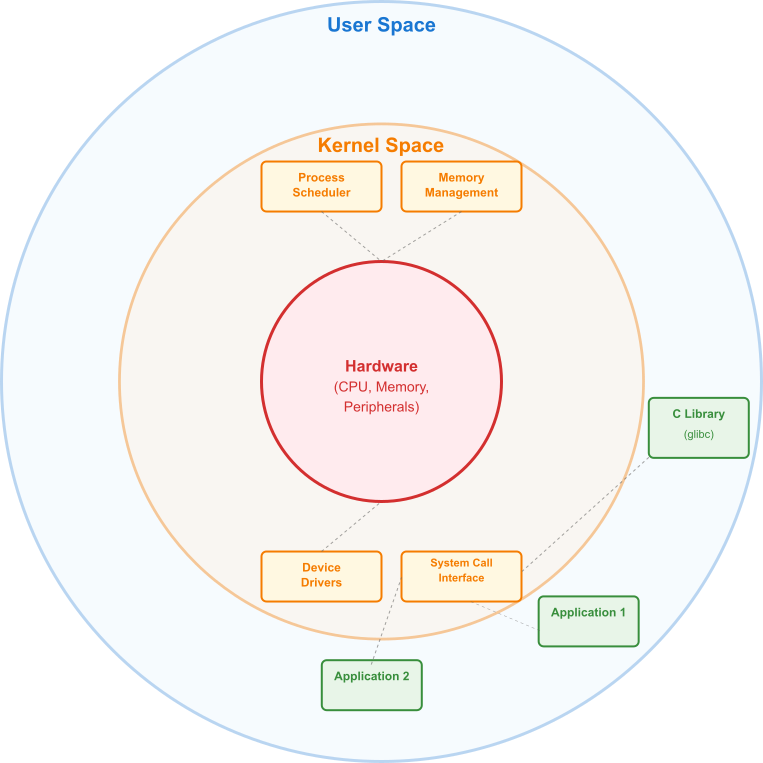
The Mountain of Abstraction: System Complexity

The power of embedded Linux comes from its layers of abstraction, which shield the application developer from the messy details of the underlying hardware. This is a double-edged sword. While the abstractions provide portability and ease of use, they also create a formidable mountain of complexity that can be daunting for newcomers and even experienced engineers. The learning curve for building, configuring, and maintaining a custom embedded Linux system is notoriously steep.

From Bootloader to Kernel

This complexity begins at the lowest level: the bootloader. On platforms like the Raspberry Pi, the process is somewhat hidden, but in a custom hardware design, the developer is responsible for the bootloader, typically U-Boot (Das U-Boot). The bootloader is a mini-OS in its own right, responsible for initializing the DRAM, setting up clocks, and loading the Linux kernel into memory. Configuring and porting U-Boot to a new board is a complex task requiring intimate knowledge of the SoC’s hardware.

Next is the kernel itself. The Linux kernel is highly configurable, with thousands of options that can be enabled or disabled through tools like menuconfig. A developer must choose the correct SoC support, enable the right drivers for the board’s peripherals (Ethernet, I2C, SPI, etc.), and configure core kernel features. Making the wrong choice can result in a kernel that doesn’t boot, or worse, a system that is unstable and subtly broken. Compounding this is the concept of the Device Tree, a data structure passed from the bootloader to the kernel that describes the hardware layout of the board. Writing and debugging a Device Tree Blob (DTB) requires careful reading of datasheets and a precise understanding of its syntax.

The Vastness of User Space and Build Systems

Beyond the kernel lies the vast expanse of user space. Here, the complexity explodes. A developer must choose a C library, an init system (systemd, SysVinit, etc.), and a selection of libraries and applications for the root filesystem. How do you build all of this from source? This is where professional-grade build systems like the Yocto Project and Buildroot come in. These are not simple tools; they are incredibly powerful and complex frameworks. The Yocto Project, for example, is a complete development environment that uses a collection of “recipes” to fetch, configure, compile, and package thousands of different open-source components into a cohesive, custom Linux distribution. Learning its syntax, concepts (layers, recipes, machine configurations), and workflow can take weeks or months. Buildroot is simpler, focusing on generating a single root filesystem image, but it is still a complex system that requires significant effort to master.

This complexity stands in stark contrast to the RTOS world, where a developer typically works with a single vendor’s toolchain, and the entire OS and application are compiled and linked into a single executable image. In the Linux world, the system is composed of hundreds or thousands of independently compiled parts, and managing their dependencies, versions, and configurations is a major engineering challenge in itself. Debugging is also more complex. A problem could be in the application, a shared library, the kernel, a device driver, the device tree, or the bootloader. It requires a holistic understanding of the entire system to effectively track down and solve issues.

flowchart TD
    subgraph "Developer's Workstation"
        A[Start: Project Requirements] --> B{Choose Build System};
        B --> C[Buildroot];
        B --> D[Yocto Project];

        subgraph "Buildroot Path"
            C --> C1[<br>1. make menuconfig<br><i>Configure system</i>];
            C1 --> C2[<br>2. make<br><i>Build all components</i>];
            C2 --> C3[<br>3. output/images<br><i>Get sdcard.img</i>];
        end

        subgraph "Yocto Project Path"
            D --> D1["<br>1. Configure local.conf<br><i>Set machine, distro</i>"];
            D1 --> D2["<br>2. Add/Create Layers<br><i>Customize BSP, apps</i>"];
            D2 --> D3["<br>3. bitbake core-image-minimal<br><i>Build image</i>"];
            D3 --> D4["<br>4. deploy/images<br><i>Get .wic image, packages</i>"];
        end
    end

    subgraph "Deployment"
        C3 --> E{Flash to Target};
        D4 --> E;
        E --> F[Embedded Device Boots];
    end

    %% Styling
    classDef startNode fill:#1e3a8a,stroke:#1e3a8a,stroke-width:2px,color:#ffffff
    classDef decisionNode fill:#f59e0b,stroke:#f59e0b,stroke-width:1px,color:#ffffff
    classDef processNode fill:#0d9488,stroke:#0d9488,stroke-width:1px,color:#ffffff
    classDef endNode fill:#10b981,stroke:#10b981,stroke-width:2px,color:#ffffff

    class A startNode;
    class B decisionNode;
    class C,D,C1,C2,D1,D2,D3 processNode;
    class C3,D4,E processNode;
    class F endNode;

The Fine Print: Licensing and Legal Obligations

Embedded Linux is built upon the foundation of the open-source software movement, and with that comes a set of legal obligations that are critical for any commercial project.

The GNU GPLv2 and Its “Copyleft” Nature

The Linux kernel itself is licensed under the GNU General Public License, version 2 (GPLv2). The GPL is a “copyleft” license, a clever play on the word “copyright.” Unlike permissive licenses (like MIT or BSD) that allow you to do almost anything with the code, a copyleft license comes with specific requirements.

The central tenet of the GPLv2 is that if you distribute a binary work that is derived from GPLv2-licensed code (a “derivative work”), you must also make the “Corresponding Source” code available to the recipients of your binary. In the context of the Linux kernel, this means if you ship a product containing a device with the Linux kernel on it, you are obligated to provide the complete source code for that specific version of the kernel, including any modifications you have made, to anyone who receives the product. This allows them to recompile and reinstall the kernel on their device.

graph TD
    A[Start: Develop Product with Linux] --> B{Is the code part of the<br>Linux Kernel or a derived work?};
    
    B -- "Yes (e.g., Kernel module, patch)" --> C[You MUST provide the<br>complete Corresponding Source<br>under GPLv2];
    B -- "No (e.g., User-space application<br>using syscalls)" --> D{Does your app link against<br>a GPL/LGPL library?};

    D -- "No (e.g., static binary, MIT libs)" --> E[GPL obligations from kernel<br>do not extend to your app.<br>Comply with other licenses.];
    D -- "Yes, links against LGPL lib<br>(e.g., glibc dynamically)" --> F[Provide a way for user to<br>re-link your app with a modified<br>version of the LGPL library.];
    D -- "Yes, links against GPL lib" --> G[Your application is now a<br>derivative work of that library.<br>You MUST release your app's<br>source under the GPL.];

    C --> H((End: Compliance Met));
    E --> H;
    F --> H;
    G --> I((End: Compliance Met - App is Open Source));

    %% Styling
    classDef startNode fill:#1e3a8a,stroke:#1e3a8a,stroke-width:2px,color:#ffffff
    classDef decisionNode fill:#f59e0b,stroke:#f59e0b,stroke-width:1px,color:#ffffff
    classDef processNode fill:#0d9488,stroke:#0d9488,stroke-width:1px,color:#ffffff
    classDef endNode fill:#10b981,stroke:#10b981,stroke-width:2px,color:#ffffff
    classDef warnNode fill:#ef4444,stroke:#ef4444,stroke-width:1px,color:#ffffff

    class A startNode;
    class B,D decisionNode;
    class C,E,F processNode;
    class G warnNode;
    class H,I endNode;

Navigating the Broader License Ecosystem

This requirement often causes concern in the corporate world, where protecting intellectual property (IP) is paramount. A common misconception is that using Linux forces you to open-source your entire application. This is generally not true. The GPLv2’s obligations are typically understood to apply to the kernel itself (kernel space) and other GPL-licensed programs in user space. Your proprietary, closed-source applications running on top of the OS (in user space) are generally not considered derivative works of the kernel, as they interact with it through well-defined system calls. This is a crucial distinction. You can write a proprietary application that runs on Linux without having to release its source code.

However, the complexity arises from the fact that your root filesystem will contain many other components with various licenses. Some, like the GNU C Library (glibc), may be licensed under the LGPL (Lesser General Public License), which has different requirements for linking. Others may use permissive MIT, BSD, or Apache licenses. A commercial product may contain hundreds of open-source packages, and the development team is legally responsible for understanding and complying with the terms of every single one. This involves conducting a license audit, generating a manifest of all software and their licenses, and ensuring that all obligations, such as providing source code and attribution notices, are met. Failure to do so can lead to legal action and a damaged corporate reputation. For companies accustomed to proprietary software development, this is a significant and often underestimated aspect of adopting embedded Linux.

Practical Examples

Theory provides the foundation, but practical application solidifies understanding. In this section, we will use the Raspberry Pi 5 to explore the challenges we’ve discussed. We will measure the resource footprint of a standard OS, witness the effects of kernel latency, and simulate the process of building a minimal system to appreciate the complexity involved.

Warning: Always back up your primary SD card before writing new images to it. These examples involve overwriting the SD card, which will erase all existing data.

Example 1: Analyzing the Resource Footprint of Raspberry Pi OS

Raspberry Pi OS is a fantastic, full-featured distribution, but its convenience comes at the cost of resources. Let’s quantify this.

1. Hardware Setup:

• A Raspberry Pi 5 with a power supply.
• An SD card flashed with the latest 64-bit Raspberry Pi OS (Desktop version).
• A monitor, keyboard, and mouse connected to the Pi.

2. Procedure: Measuring Usage

First, boot your Raspberry Pi 5 into the desktop environment. Open a terminal window and execute the following commands.

Check Memory (RAM) Usage: The free command provides a snapshot of RAM usage. The -h flag makes the output “human-readable.”

free -h


Expected Output (will vary):

              total        used        free      shared  buff/cache   available
Mem:          7.8Gi       1.2Gi       5.8Gi       112Mi       850Mi       6.4Gi
Swap:         100Mi          0B       100Mi


Explanation: Even at idle on the desktop, the system is using over a gigabyte of RAM! The buff/cache value shows memory used for disk caching, which can be reclaimed if needed. The truly “used” figure is a combination of application and system processes.

Check Storage (Disk) Usage: The df command reports filesystem disk space usage.

df -h /


Expected Output (will vary):

Filesystem      Size  Used Avail Use% Mounted on
/dev/root        29G  7.5G   21G  28% /


Explanation: A fresh installation of Raspberry Pi OS with a desktop environment consumes around 7-8 GB of storage space. This is a massive footprint for many embedded applications.

View Running Processes: The top command provides a real-time view of running processes and their resource consumption.

top


Press q to exit. You will see a long list of processes, from the X11 display server to various desktop services and background daemons, all consuming CPU cycles and RAM.

3. Building a Minimalist System with Buildroot

Now, let’s contrast this with a truly embedded approach. We will use Buildroot on a separate Linux host machine (e.g., Ubuntu 22.04) to build a minimal image for our Raspberry Pi 5.

Build and Configuration Steps (on a Linux Host PC):

Install Prerequisites:

sudo apt update
sudo apt install -y build-essential libncurses-dev rsync wget unzip bc

Download and Extract Buildroot:

wget https://buildroot.org/downloads/buildroot-2024.05.tar.gz
tar -xf buildroot-2024.05.tar.gz
cd buildroot-2024.05/

Configure for Raspberry Pi 5: Buildroot includes a default configuration for the Pi 4, which we can adapt for the Pi 5.

make raspberrypi4_64_defconfig

Customize the Configuration: This is the crucial step for minimizing the footprint. We’ll use menuconfig, a text-based configuration interface.

make menuconfig


Navigate the menus using the arrow keys. Here are a few things to change to create a minimal system:

• Target packages —>
  • Deselect [ ] Audio and video applications

• • Deselect [ ] Games

• • Deselect [ ] Graphic libraries and applications (graphic stack)

• • Under [ ] Networking applications, deselect everything except what is essential (e.g., keep dropbear for SSH).
  Filesystem images —>
  • Ensure [ ] ext2/3/4 root filesystem is selected.

• • Set (120) to ext2/3/4 root filesystem size in MB. Let’s make it small, like 120 MB.

Build the Image: This process will take a long time (30 minutes to several hours) as it downloads and compiles the entire toolchain, kernel, and user space from scratch.

make

Flashing and Booting:

Once the build completes, the final image will be located at output/images/sdcard.img.

Use a tool like dd or Raspberry Pi Imager to flash this sdcard.img file to your SD card.

Warning: Ensure you specify the correct device for your SD card (e.g., /dev/sdX). Using the wrong device will destroy data on that drive.

# Example using dd. Find your SD card with `lsblk`.
sudo dd if=output/images/sdcard.img of=/dev/sdX bs=4M conv=fsync

Insert the SD card into your Raspberry Pi 5 and power it on. Connect a serial-to-USB adapter to the Pi’s UART pins (GPIO 14/15) to see the boot messages.

Expected Outcome:

The Pi will boot to a simple login prompt on the serial console. Log in with the username root (no password by default). Now, run the same commands:

• free -h: You will see memory usage in the tens of megabytes, not gigabytes.
• df -h: The entire root filesystem will be using less than 100 MB of space.

This dramatic difference showcases the resource challenge: the default experience is convenient but bloated, while the embedded approach is efficient but requires significant effort and complexity to build.

Example 2: Visualizing Real-Time Latency

This example demonstrates the non-determinism of a standard kernel. We will write a C program to toggle a GPIO pin as fast as possible and observe the timing jitter.

1. Hardware Setup:

• A Raspberry Pi 5 running standard Raspberry Pi OS.
• An oscilloscope or logic analyzer.
• A jumper wire.
• Connect the probe of your measurement device to GPIO 17 (Pin 11) and the ground probe to a ground pin on the Pi.

2. Code Snippet: gpio_toggle.c

We will use the gpiod library, which is the modern way to interact with GPIOs on Linux.

// gpio_toggle.c
// Toggles a GPIO pin as fast as possible to demonstrate latency.
// Compile with: gcc -o gpio_toggle gpio_toggle.c -lgpiod

#include <gpiod.h>
#include <stdio.h>
#include <unistd.h>
#include <time.h>

#ifndef	CONSUMER
#define	CONSUMER	"gpio_toggle"
#endif

int main(int argc, char **argv)
{
	char *chipname = "gpiochip4"; // GPIOs on RPi 5 are on chip 4
	unsigned int line_num = 17; // GPIO 17
	struct gpiod_chip *chip;
	struct gpiod_line *line;
	int i, val = 0;

	// Open the GPIO chip
	chip = gpiod_chip_open_by_name(chipname);
	if (!chip) {
		perror("Open chip failed");
		return 1;
	}

	// Get the GPIO line
	line = gpiod_chip_get_line(chip, line_num);
	if (!line) {
		perror("Get line failed");
		gpiod_chip_close(chip);
		return 1;
	}

	// Request the line for output
	if (gpiod_line_request_output(line, CONSUMER, 0) < 0) {
		perror("Request line as output failed");
		gpiod_line_release(line);
		gpiod_chip_close(chip);
		return 1;
	}

	printf("Toggling GPIO %d on %s. Press CTRL-C to exit.\n", line_num, chipname);

	// Toggle the pin in a tight loop
	while (1) {
		val = !val;
		if (gpiod_line_set_value(line, val) < 0) {
			perror("Set line value failed");
			break;
		}
	}

	// Release resources
	gpiod_line_release(line);
	gpiod_chip_close(chip);

	return 0;
}

3. Build and Run Procedure:

• Install libgpiod:

sudo apt update
sudo apt install -y gpiod libgpiod-dev

• Compile the code:

gcc -o gpio_toggle gpio_toggle.c -lgpiod

• Run the program and observe:

./gpio_toggle

Expected Output on Oscilloscope/Logic Analyzer:

You will see a square wave. However, if you zoom in on the time axis, you will notice that the period of the wave is not perfectly consistent. You will see occasional “glitches” where a pulse is significantly longer than the others. This is jitter. These long pulses occur when the kernel preempts our gpio_toggle process to handle another task (like a network interrupt or a scheduler tick). This is a direct, visual measurement of the non-determinism of the standard kernel.

To truly see the improvement, one would need to repeat this experiment after building and installing a PREEMPT_RT kernel on the Pi. The resulting square wave would have a much more consistent period, with the ‘delta’ of the jitter being significantly smaller and more bounded. The process of building a PREEMPT_RT kernel is an advanced topic, but this simple experiment powerfully illustrates the problem it solves.

Common Mistakes & Troubleshooting

Navigating the challenges of embedded Linux development often involves learning from mistakes. Here are some common pitfalls that engineers, both new and experienced, frequently encounter.

Exercises

These exercises are designed to reinforce the concepts of resource management, system complexity, and real-time analysis on your Raspberry Pi 5.

1. Beginner: Boot Time Analysis
   • Objective: Analyze the boot process of the standard Raspberry Pi OS to identify which services consume the most time. This demonstrates the complexity of the user-space startup sequence.
   • Guidance:
     1. Boot your Raspberry Pi 5 with the standard Raspberry Pi OS.
     2. Open a terminal.
     3. The systemd-analyze tool provides detailed boot performance statistics.
     4. Run systemd-analyze to see the total boot time.
     5. Run systemd-analyze blame to get a sorted list of all services and the time they took to initialize.
   • Verification: Identify the top five longest-running services. Research what one of these services does. Does your embedded application truly need it? This exercise highlights how many non-essential services run on a desktop-oriented distribution.
2. Intermediate: Further Buildroot Minimization
   • Objective: Take the minimal Buildroot image created in the practical example and shrink it even further. This reinforces the concept of resource footprint management.
   • Guidance:
     1. Return to your Buildroot source directory on your host PC.
     2. Run make menuconfig.
     3. Dive deeper into the Target packages menu. Try disabling more features, such as all networking applications or even the login shell itself (the system will boot but you won’t be able to log in, proving it works).
     4. Explore the Toolchain ---> menu and consider switching from glibc to musl, a C library designed for static linking and smaller footprints.
     5. Rebuild the image with make.
   • Verification: Flash the new sdcard.img and check its size. Compare the size of the new image file with the one from the practical example. How small were you able to make it?
3. Advanced: Quantitative Latency Measurement with cyclictest
   • Objective: Use a standard industry tool to quantitatively measure the real-time performance of your kernel and generate a statistical report.
   • Guidance:
     1. On your Raspberry Pi 5 running standard Raspberry Pi OS, you need to install the real-time testing tools.sudo apt update sudo apt install -y rt-tests
     2. cyclictest is the premier tool for measuring kernel latency. It works by running a high-priority thread that sleeps for a specified interval, then measures the difference between the requested sleep time and the actual time it woke up. This difference is the latency.
     3. Run a simple test for 60 seconds:sudo cyclictest -t1 -p 80 -n -i 1000 -l 60000
        • -t1: Run one test thread.
        • -p 80: Set the thread priority to 80 (high).
        • -n: Use clock_nanosleep.
        • -i 1000: Base interval is 1000 microseconds (1ms).
        • -l 60000: Run for 60,000 loops (approx. 60 seconds).
   • Verification: Observe the output. cyclictest will print a summary table with columns for Min, Act, Avg, and Max latency (in microseconds). On a standard kernel under load (e.g., while moving the mouse or running dd if=/dev/zero of=/dev/null), you will see the Max latency spike into the hundreds or even thousands of microseconds. If you were to run this same test on a PREEMPT_RT kernel, the Max value would be significantly lower and more consistent, providing a quantitative measure of its improved determinism.

Summary

This chapter provided a critical perspective on the challenges of using Linux in embedded systems, balancing the optimistic view from previous chapters. By understanding these disadvantages, you are better prepared to create robust and efficient designs.

• Resource Requirements: Linux is resource-intensive compared to RTOSes, demanding more powerful processors, more RAM, and larger storage, which directly impacts product cost and power consumption.
• Real-Time Performance: The standard Linux kernel is optimized for throughput, not determinism. Achieving real-time capabilities requires the PREEMPT_RT patchset and careful system design to minimize latency and jitter.
• System Complexity: The embedded Linux ecosystem is immensely complex, involving bootloaders, kernel configuration, Device Trees, build systems (Yocto/Buildroot), and a vast user space. Mastering this complexity requires a significant investment in learning.
• Licensing: The use of open-source software, particularly the GPLv2-licensed kernel, imposes legal obligations to share source code for any distributed modifications. Proper license compliance is a critical, non-technical requirement for any commercial product.
• The Embedded Mindset: Successful embedded Linux development is about deliberate, informed choices. It involves starting with a minimal system and adding only what is necessary, rather than starting with everything and trying to remove what isn’t needed.

By grappling with these challenges, you move from being a user of embedded Linux to an architect of embedded Linux systems, capable of wielding its power responsibly and effectively.

Further Reading

1. The PREEMPT_RT Wiki: The official source for documentation on the real-time patchset. An essential resource for understanding how real-time is achieved in Linux.
   • https://wiki.linuxfoundation.org/realtime/start
2. Buildroot Official Documentation: The user manual for the Buildroot system. It is comprehensive and provides detailed explanations of its architecture and usage.
   • https://buildroot.org/docs.html
3. Yocto Project Documentation: The official documentation set for the Yocto Project. Start with the “Yocto Project Overview and Concepts Manual.”
   • https://docs.yoctoproject.org/
4. “Mastering Embedded Linux Programming, 3rd Edition” by Chris Simmonds: An excellent, up-to-date book that covers many of the practical challenges discussed in this chapter in great detail.
   • Publisher: Packt Publishing
5. “Anatomy of an Embedded Linux System” by Free Electrons (now Bootlin): A classic and highly-regarded presentation that clearly breaks down the components of an embedded Linux system. While a few years old, the core concepts remain highly relevant.
   • https://bootlin.com/doc/training/embedded-linux/
6. “Copyleft and the GNU General Public License: A Comprehensive Tutorial and Guide” by the Software Freedom Conservancy: A clear, readable guide to understanding the GPL.
   • https://sfconservancy.org/copyleft-guide/
7. Raspberry Pi 5 Datasheets and Documentation: Understanding the underlying hardware is crucial. The official documentation from the Raspberry Pi Foundation provides the ground truth for the hardware’s capabilities and configuration.
   • https://www.raspberrypi.com/documentation/